Hi Dronesonen! 😊
Last week we conducted the following efforts:
Discipline – Software:
Erik-Andre Hegna:
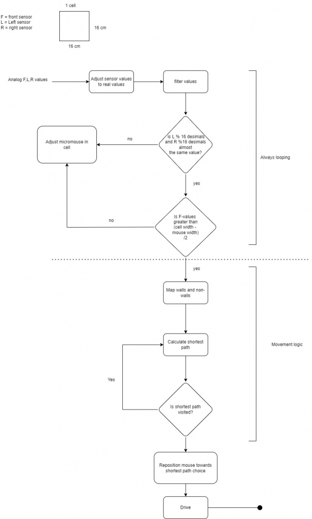
This week I focused on system modeling. My goal for this week was trying to understand how the different algorithms would work together all the way from sensor-data to moving and mapping the maze. Trying to get my head around the whole process has been challenging and fun, especially the PID.
I also spent time discussing with the group about the sensor data, how to filter it, and make it more accurate at longer ranges (the ultra sonic sensors seem to have an increasing off-set to the real range → low at close distances, bigger at longer distances).
Lars Leganger:
This week we continued working on the sensors. We want to get the sensor data filtered and accurate as possible to real world measurements. Me and ask started by finding out how much of the data we need to be accurate. We decided that the readings from 20 cm and above are not necessary to get accurate because the mouse will keep driving if the sensor does not detect something within 20 cm range. This is also good as the real measurements and signal output data varies a lot the further the distance. After that we took measurements of each cm from 1 to 20 to see how much they change and if we can add a formula that will close the gap between actual distance and sensor readings.
I also started reacherching PID controller for our mouse. The controller will allow the mouse to maintain its position in the maze.
We want a low pass filter to filter the data while in real time and not after so my job next week is to make a low pass filter for C+ that will filter constantly data that is being received. Below is how the code looks now. The filter I am trying to make is the low pass filter.
Ask Lindbråten:
The goal for this week was to improve the ultrasonic sensor reading accuracy in comparison to the real-world distances. Since I was sick on Monday, I didn’t manage to contribute anything to the group, so I met early for the session on Wednesday to hopefully catch up and have a solid day of work. I began the session by looking into the functionality of the low-pass filter Lars had worked on, and how we could apply it to smoothen a set of ultrasonic distance-measures and analyze the results using plot-graphs in Spyder.
This proved a lot more difficult then first expected, so after a few hours of troubleshooting and confusion, me and Lars decided to go with a less practical but simpler approach to visualize and analyze the captured distances from the ultrasonic sensor. We used the open rectangular box of 50 cm to note what kind of values the sensor would output for each cm in an interval of (1 to 20) cm (we imagine we could ignore every value over 20 cm since they would all result in the micromouse continuing its trajectory). Now, since we hadn’t found a way to store values to text-files using C++ and Visual Studio Code, we had to print hundreds of results to the screen and manually write down the minima and maxima values for each cm on a piece of paper… very effective, I know😐. After, noting down the min- and max-values for each cm, I wrote a script to bring those values up to they’re corresponding real-world distances. The script and the results, when running it, is pasted below:
double adjDistToRW(double n) {
    double adj_dist = 0;
        if (n >= 1.03 and n < 1.39) { // RW dist = 1
            adj_dist = std::floor(n);
            return adj_dist;
        }
        if (n >= 1.39 and n <= 1.41) { //RW dist = 2
            adj_dist = std::ceil(n);
            return adj_dist;
        }
        if (n >= 1.71 and n <= 2.33) { //RW dist = 3 -> 4
            adj_dist = std::ceil(n) + 1;
            return adj_dist;
        }
        if (n >= 2.92 and n <= 6.55) { //RW dist = 5 -> 9
            if (n == 6.09) {
                adj_dist = std::floor(n) + 3;
                return adj_dist;
            }
            else {
                adj_dist = std::ceil(n) + 2;
                return adj_dist;
            }
        }
        if (n >= 7.55 and n <= 10.58) { //RW dist = 10 -> 14
            if (n == 8.13 or n == 7.55) {
                adj_dist = std::ceil(n) + 2;
                return adj_dist;
            }
            else {
                adj_dist = std::ceil(n) + 3;
                return adj_dist;
            }
        }
        if (n >= 10.65 and n <= 12.52) { // RW dist = 15 -> 17
            if (n == 12.07) {
                adj_dist = std::ceil(n) + 3;
                return adj_dist;
            }
            else {
                adj_dist = std::ceil(n) + 4;
                return adj_dist;
            }
        }
        if (n >= 12.55 and n <= 14.53) { // RW dist = 18 -> 20
            if (n == 14.01) {
                adj_dist = std::floor(n) + 5;
                return adj_dist;
            }
            else {
                adj_dist = std::ceil(n) + 5;
                return adj_dist;
            }

        }
}
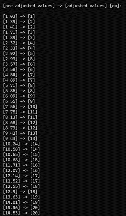
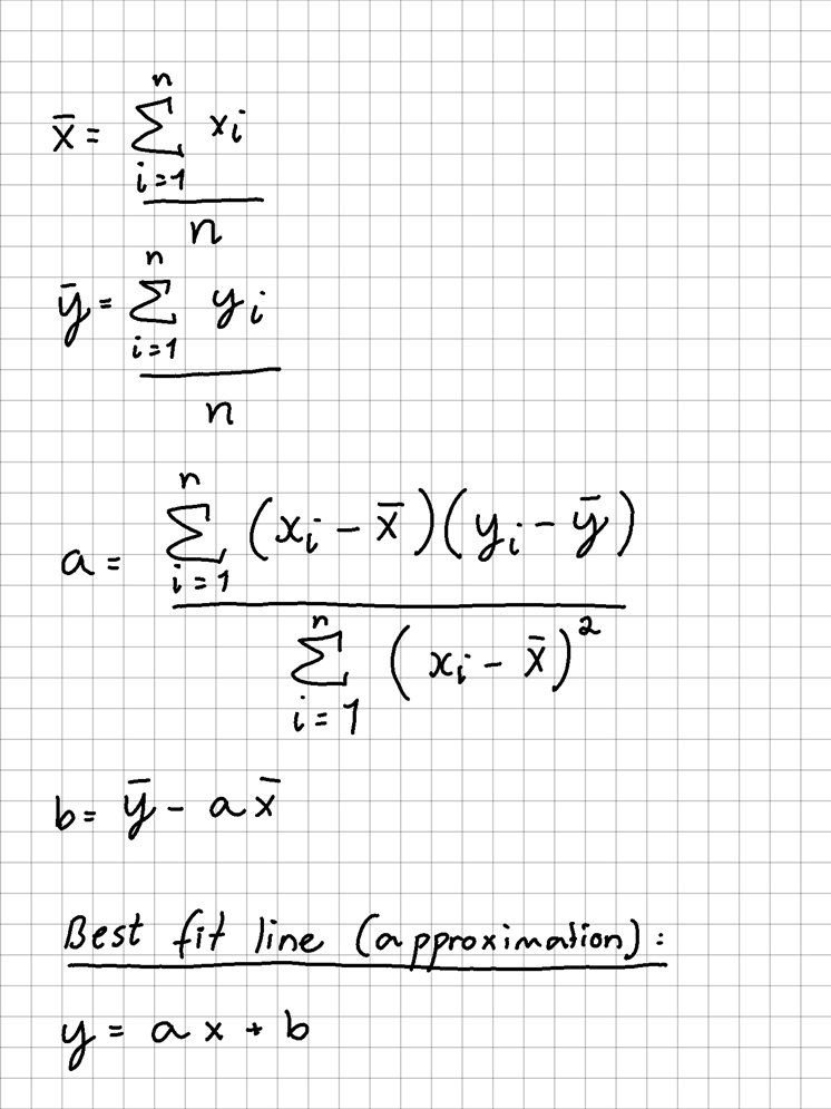
This script is of-course very “hard-coded”, so I imagine it would need an awful lot of maintenance to be able to adjust distance-values that is not calculated under “perfect” test-conditions, or where the real-world distance is not a whole number. Therefore, I decided to use the data I had written down, plot them in GeoGebra, and calculate a best fit linear function where measurement “x” is inputted to find the approximate corresponding real-world distance “y”. I used the least square method, and ran the following equations in Visual Studio to calculate a best fit linear function y(x):
int main()
{

    std::vector<double> pre_adj_dist_vals{ 1.03, 1.39, 1.41, 1.71, 1.89, 2.32, 2.33,
                                          2.92, 2.93, 3.57, 3.58, 4.54, 4.89, 5.71, 5.85, 6.09,
                                          6.55, 7.55, 7.75, 8.13, 8.68, 8.73, 9.42, 9.43, 10.24, 10.58,
                                          10.65, 10.68, 11.71, 12.07, 12.14, 12.52, 12.55, 12.90, 13.63,
                                          14.01, 14.46, 14.53 };

    std::vector<double> adj_dist_vals{};
    std::vector<double> RW_records{ 1, 2, 2, 3, 3, 4, 4, 5, 5,
                                    6, 6, 7, 7, 8, 8, 9, 9, 10,
                                    11, 11, 12, 12, 13, 13, 14, 14,
                                    15, 15, 16, 16, 17, 17, 18, 18,
                                    19, 19, 20, 20 };
double measures_sum = 0;
double num_of_measures = pre_adj_dist_vals.size();
double mean_measures = 0;

for (int i{ 0 }; i < pre_adj_dist_vals.size(); i++) {
    measures_sum += pre_adj_dist_vals[i];
}
mean_measures = measures_sum / num_of_measures;

double RW_records_sum = 0;
double num_of_RWrecordings = RW_records.size();
double mean_records = 0;

for (int i{ 0 }; i < pre_adj_dist_vals.size(); i++) {
    RW_records_sum += RW_records[i];
}

mean_records = RW_records_sum / num_of_RWrecordings;

double rate_of_increase = 0;
double diff_measures = 0;
double diff_records = 0;
double diff_total = 0;

for (int i{ 0 }; i < num_of_measures; i++) {
    diff_total += (pre_adj_dist_vals[i] - mean_measures) * (RW_records[i] - mean_records);
}

double diff_measures_squared = 0;

for (int i{ 0 }; i < num_of_measures; i++) {
    diff_measures_squared += std::pow((pre_adj_dist_vals[i] - mean_measures), 2);
}

rate_of_increase = (diff_total) / diff_measures_squared;
double y_intcpt = mean_records - (rate_of_increase * mean_measures);
std::cout << "y = " << rate_of_increase << "x + " << y_intcpt;
}
Running the script gave me the following line:

Below is the line plotted in GeoGebra along with a table of the points. The x-axis has the measured distances, and the y-axis has the approximate corresponding real-world distances.
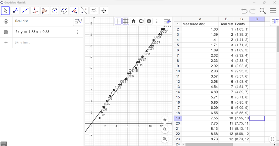
We still need to plot a lot more values this week/the following weeks and under various test conditions, so we can develop the best approximate function to correctly map and make the right actions in the maze.
Discipline – Electrical:
Hugo Valery Mathis Masson-Benoit:
The objective for this week was to start the design for the encoders.
Sensor part:
This week the software engineers all agreed for the use of ultrasonic sensor to replace the IR ones. We’re going to use three ultrasonic sensors instead of four IR sensors. They are now testing with it, and I’m helping when they need me.
Encoder part:
The magnetic sensor and some little magnets have been ordered this week to create the encoders. There should be delivered next week for us to work with.
On the other hand, the software engineers are not sure if they need encoders, so maybe it won’t be a problem. But we can’t be sure, so I’m working on it either way.
Conclusion:
The hardware of the Micromouse is almost finished, the sensor is chosen, the motors also, and only the encoders are left to do. But we need to have the structure of the mouse to work with.
Objective for next week:
Finish the electronic design and start the PCB design in accordance with the mechanical engineer.
Discipline – Mechanical:
Cesia Niquen Tapia & Jemima Niquen Tapia:
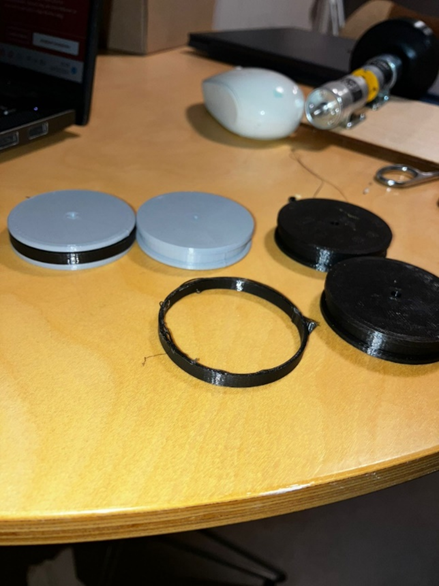
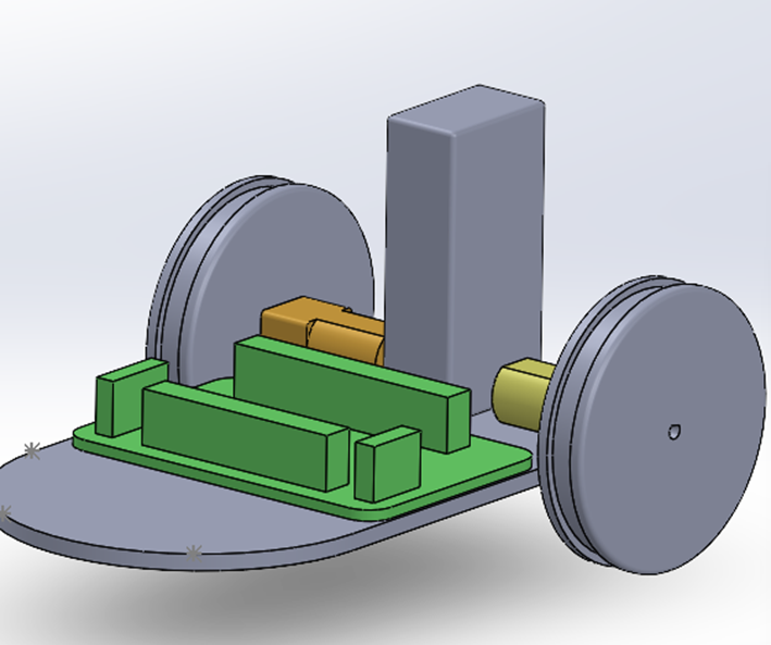
This week there was an important change in the components of our micromouse and this leads to a change of the structure. We got new engines, smaller , and also without a supporter. So, we had to design a new supporter, new wheels and also a new chassis according to this new dimensions.
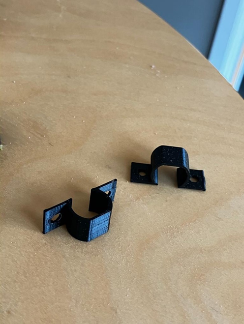
Also, for code trial we needed the new tractional design for the old engines, so we printed the same new ones but with the respective dimensions.
This concludes our blog post for week 8, see you next week!😊