Hey there, Blogz fam! 🌟

Another week has flown by, and let me tell you, it’s been quite the rollercoaster! 🎢 But, as always, we’ve been working tirelessly to bring our Turret System project to life. 💪

Now, let’s dive right in and see what each of our amazing team members has been up to this week, all contributing their unique talents to make our dream a reality! 🚀

Stay tuned as we unveil the magic behind our Turret System! 🔮💼

Harald Berzinis

Trigger Mechanism 

Concept

Safety and precision were at the forefront of our design philosophy. Our goal? Develop a mechanism ensuring the paintball gun fires a single shot, necessitating manual reloading thereafter. This approach not only reduces the risk of unintentional continuous firing but also brings a human element back to the autonomous paintball turret.

Mechanism Details

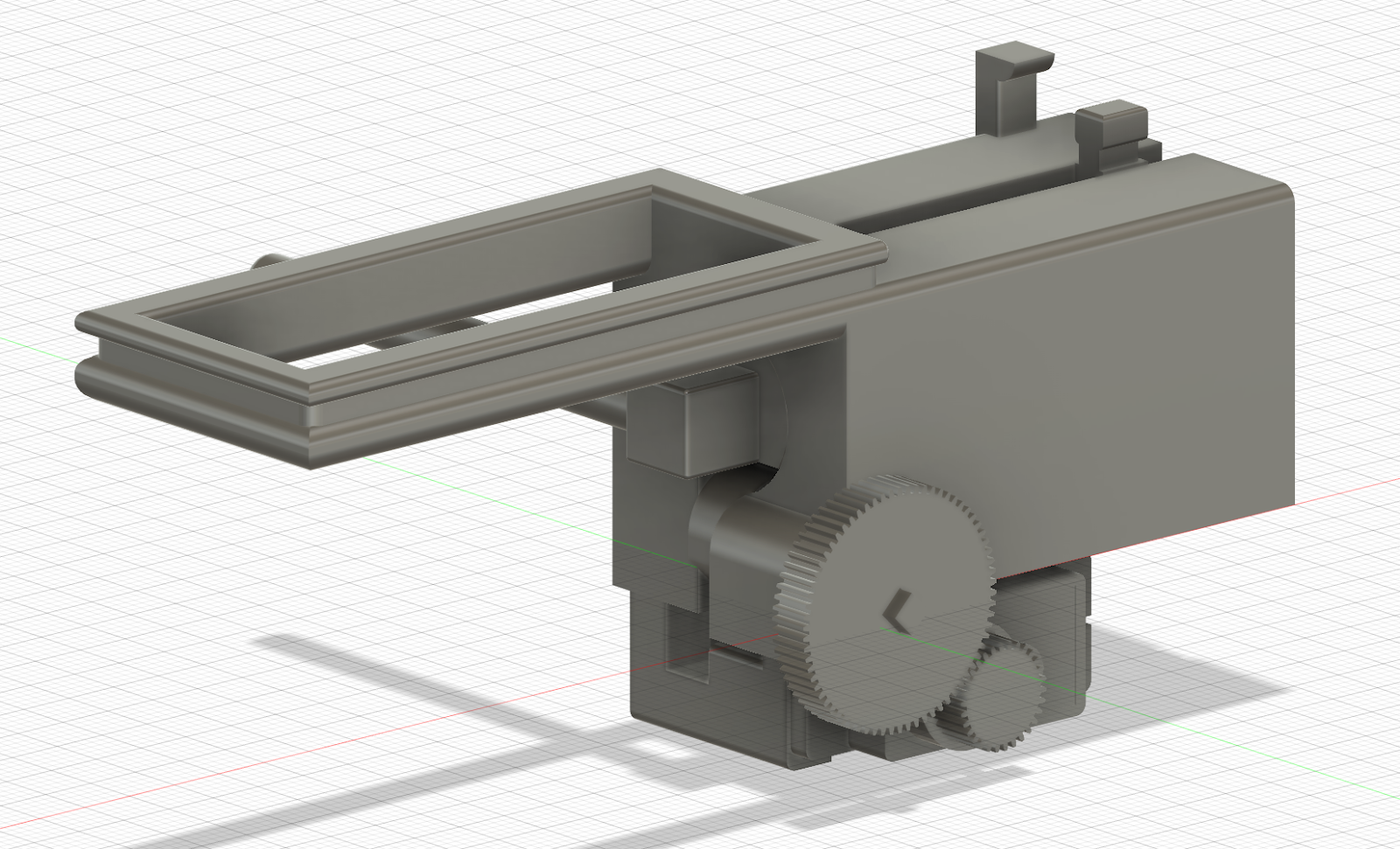
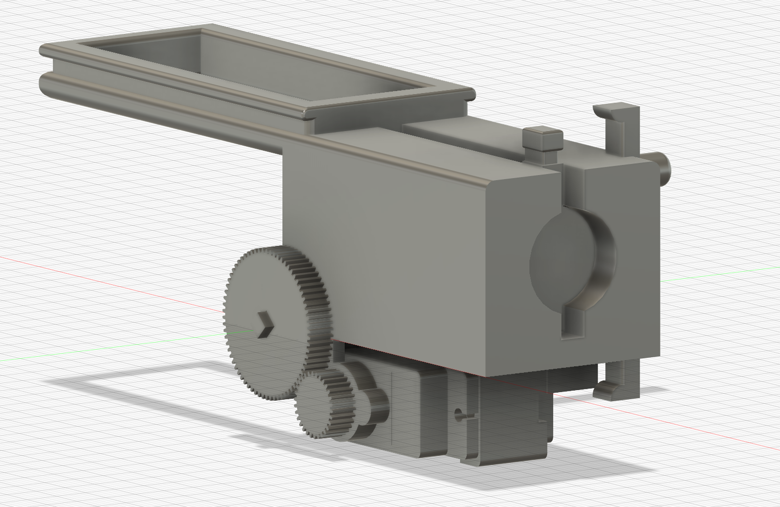
Central to our design is a bolt propelled by untraditional rubber bands. Upon activation, this bolt engages the trigger, releasing a shot from the paintball gun. Moving beyond the bolt design, the driving force behind this bolt is a SG90 servo and some gears.

Operational Dynamics

The SG90 servo functions through a set of interconnected gears. Working in harmony, these gears convert the servo’s inherent rotational motion into the required linear action, powering the bolt’s forward thrust to activate the trigger.

Assembly & Mounting

3D printing technology enabled the meticulous crafting of each component. Once printed, these parts should fit together and secured with a robust adhesive. To streamline the mounting process, the design integrates dedicated zip-tie slots. This ensures that the mechanism can be both swiftly and stably affixed to the paintball gun. Further enhancing stability, the SG90 servo is anchored using a pair of screws, eliminating the necessity for additional adhesives.

Screenshots of the trigger mechanism in Fusion 360

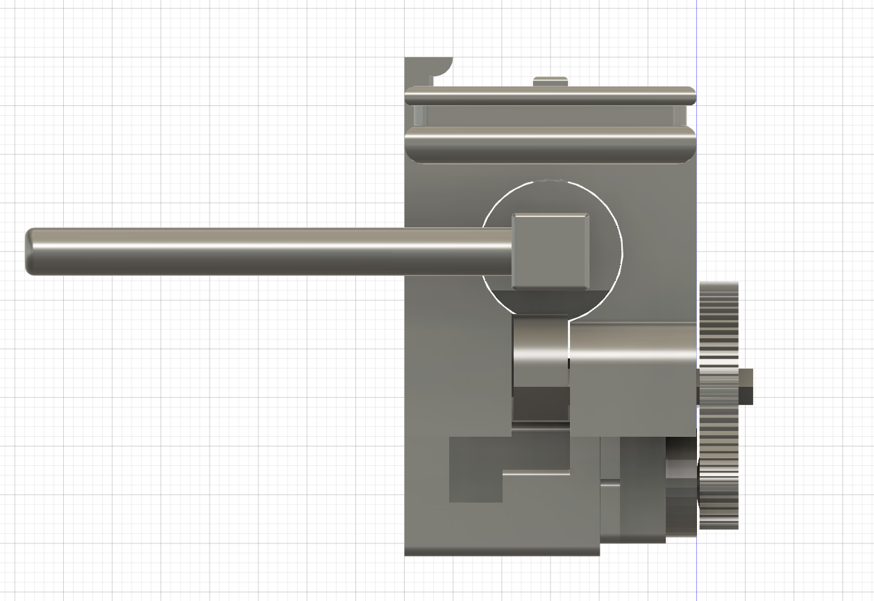
The bolt mechanism will be tensioned with rubber bands

Summary and next week

Our trigger mechanism, conceived with a clear focus on safety and operational efficiency, strikes a perfect balance between automation and human engagement. Furthermore, the plan for the next week is further improving the contraption and start printing the first prototype.

Mats Bergum

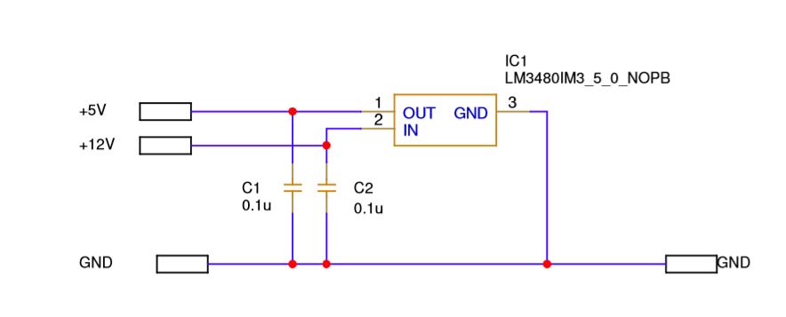
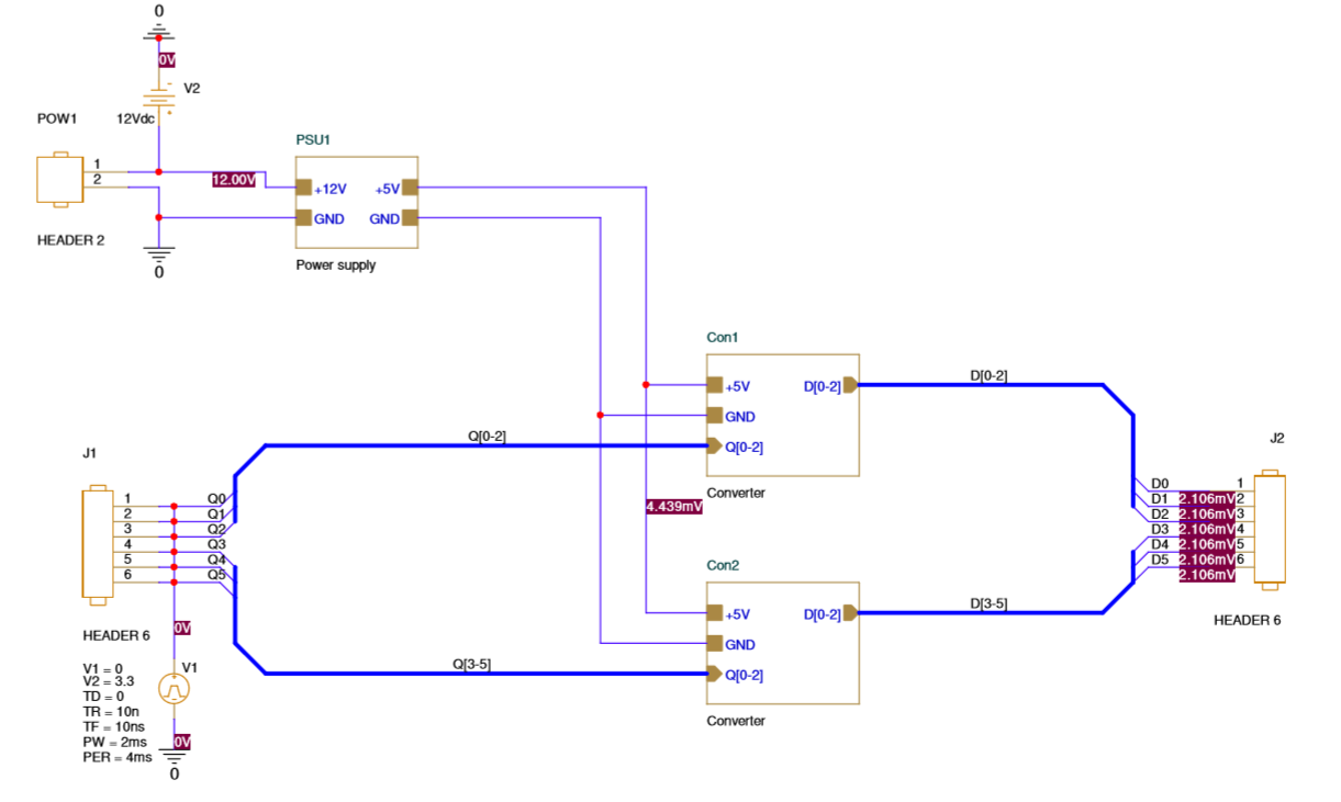
Started making PSU subcircuit using the  LM3480IM3-5.0/NOPB integrated circuit (IC) from Texas Instrument. The circuit used was changed from the one produced by Harald. Since the original component was not available. Moreover, LM3480IM3-5.0/NOPB gives a more reliable supply of 5V than LM317D2TR4G. This subcircuit delivers +5V for the converter circuits and the +5V output. The PSU circuit can be found in the figure below.

Afterward, I made the converter circuit. The circuit can be found below. This is precisely the same design as the one made by Harald. Then, using Pspice, the circuit was tested using a pulse of 250Hz with an amplitude of 3.3V for the input (Q[0-2]).

This is 50Hz higher than what is required for practical use. The waveform can be found below.

As you can see from the figure, there is a slight fall time for the output, but it is not big enough to make an impact. 

Then, I put all the subcircuits together, as shown below. Not that there may be some changes to this circuit when I design the PCB next week.

By using Pspice, the complete circuit was tested.

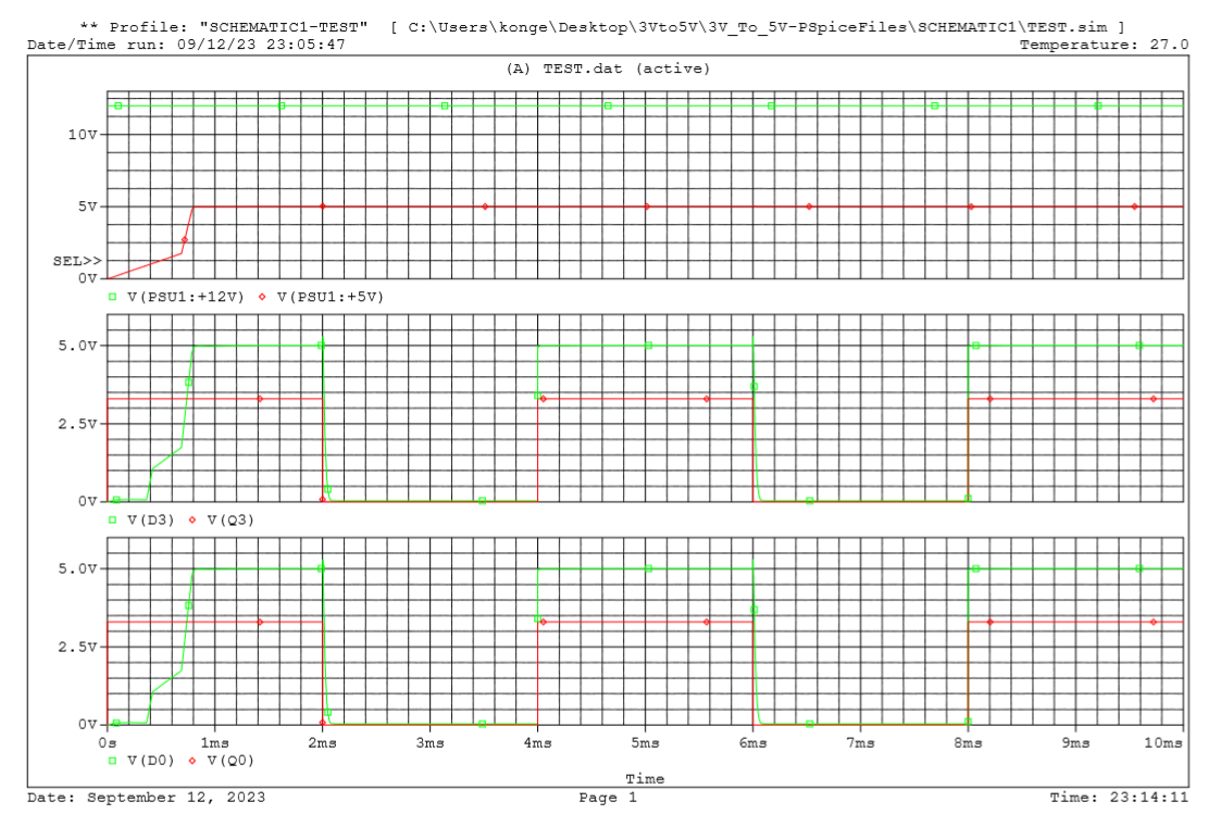
The only thing to note is that the +5V output uses a short time to set, but it is only for 0.8ms initially, so it is not a problem. 

Next week I plan to complete the PCB design and prepare it for printing. Of course, some problems may occur since I have no experience making a PCB design.

Christopher Daffinrud

This week my focus was on developing a high-level architectural design for our forthcoming software implementation.

The structure was created by drawing upon our preliminary research around our previous function-analysis of the system and our experimentation with color identification, object recognition using trained models with EfficientDet Tensorflow Lite and our motor controllers.

I created the following object-oriented class diagram to serve as a foundation structure for our software implementation. 

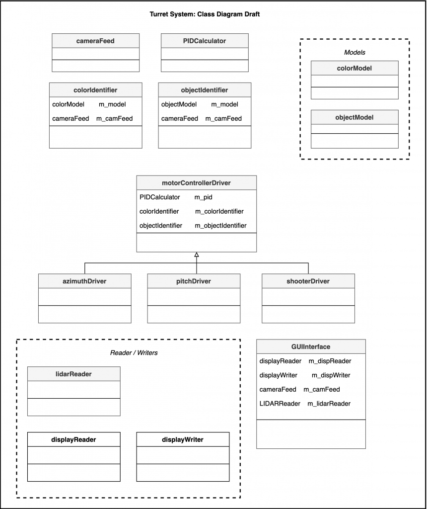
Both the colorIdentifier and objectIdentifier classes now include an instance of the cameraFeed. This decision was made to provide us with the flexibility to test resource utilization: If it is less demanding identifying the color before the object or vice versa. 

It’s important to note in the diagram that the GUI Interface-class is considered a preliminary iteration. Depending on the resources available to us on the Pi, and further testing of our resources, we may need to look at alternatives for our GUI. We have also looked at the possibility of maybe integrating a web based application in our system using Flask.

Next week I will continue to iterate on the architectural design and map out different methods needed for our systems functional requirements.  

Ole Eirik S.Seljordslia

After successfully installing an older version of OpenVino last week, we unfortunately discovered that it was dependent on OpenVino development tools packages to run inference for models. However, we encountered difficulties while attempting to install this dev tools package on the Raspberry Pi.

At this point, we had already invested a significant amount of time trying to make the Compute Stick 2 work with the Raspberry Pi. Consequently, I decided to explore an alternative approach by using smaller object detection models. After conducting some research, I came across the TensorFlow Lite library, which is designed for deploying models on mobile devices, microcontrollers, and other edge devices. This appeared to be a viable option, especially since there was an example of object detection for the Raspberry Pi 4 within the library’s documentation.

The example provided by TensorFlow yielded satisfactory results. We were able to detect objects from the COCO2017 dataset at a rate of approximately 6-10 frames per second while utilizing all four cores of the Raspberry Pi. However, the Pi’s CPU temperature quickly rose to 80 degrees, prompting us to realize the need for active cooling if we intended to use it with the Raspberry Pi.

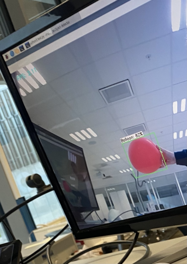
Given that this was the most promising result we had achieved for object detection, I decided to dedicate the rest of the week to finding an optimal detection model that could provide both precision and speed, specifically for detecting balloons at distances of 5-10 meters and at a rate of around 10 frames per second. To test the Raspberry Pi’s capabilities, we used the EfficientDet(also used in previously mentioned example) model, which exists in various versions offering different tradeoffs between precision and speed. To achieve balloon detection, I needed to retrain the model using images of balloons.

For model retraining, we required images that provided information about the location of the object the model aimed to detect. After browsing Kaggle, I discovered a simple dataset consisting of 74 images of balloons, which appeared to be a suitable starting point for building our dataset. TensorFlow offers an example of how to retrain a model and convert it into a TensorFlow Lite model. In this example, they use approximately 100 images to train the model on five different classes.

However, training the model introduced a new set of dependency challenges. None of the available versions of the tflite_model_maker were compatible with the Python version or the architecture of either the Raspberry Pi or my laptop. As training required significant computational resources and specific dependencies, I decided to use Google Colab in order to train the model and mitigate the challenges regarding dependencies and python versions.

I created a Jupyter notebook to ensure the correct Python version by downgrading the IPython kernel and installing the specific dependencies required for tflite_model_maker. The Jupyter notebook also handled the splitting and transformation of the dataset. Each image had to be categorized as either train, test, or validation, which was done randomly. The original dataset utilized a CSV file to specify the locations of the bounding boxes for the balloons within the images. This information needed to be transformed into a new CSV file that adhered to TensorFlow’s object detection dataloader format.

The following code block converts from the kaggle dataset format to tensorflow’s format: 

Kaggle dataset format

Tensorflow format

 1
 2
 3
 4
 5
 6
 7
 8
 9
10
11
12
13
14
15
16
17
18
19
20
21
22
23
24
25
26
27
28
29
30
31
32
33
34
35
36
37
38
39
40
41
42
43
44
45
46
47
48

classes = ['Balloon']
images = os.listdir('dataset/images')
number_of_images = len(images)
train_percent = 0.8
validation_percent = 0.1
test_percent = 0.1
# Python will always round down, test_number_images gets the remaining images
train_number_of_images = int(number_of_images * train_percent)
validation_number_of_images = int(number_of_images * validation_percent)
test_number_of_images = number_of_images - train_number_of_images - validation_number_of_images
def relative_coordinate(maximum: int, value: int):
   return np.float32(value/maximum)[0]
def move_files(amount: int, label: str, images: list):
  path = rf'dataset/{label}'
  all_meta = pd.read_csv(rf'dataset/balloon-data.csv')
  all_meta['bbox'] = all_meta['bbox'].apply(ast.literal_eval)
  print(f'Moving {amount} files to {path}')
  meta = pd.DataFrame(columns=['label', 'path', 'class', 'x_min', 'y_min','dummy','dummy',
                              'x_max', 'y_max', 'dummy', 'dummy'])
  for i in range(amount):
      file = random.choice(images)
      print(rf'dataset/images/{file}')
      print(rf'{path}/{file}')
      entry = all_meta.loc[all_meta['fname'] == file]
      for boxes in entry['bbox']:
        for box in boxes:
          meta.loc[len(meta)] = {'label': label.upper(), 'path': rf'{path}/{file}', 'class': 'Balloon',
                       'x_min': relative_coordinate(entry['width'] ,box['xmin']),
                       'y_min': relative_coordinate(entry['height'], box['ymin']),
                       'x_max': relative_coordinate(entry['width'], box['xmax']),
                       'y_max': relative_coordinate(entry['height'], box['ymax'])}
      shutil.copy(rf'dataset/images/{file}', rf'{path}/{file}')
      images.remove(file)
  return meta, images
train_meta_data, images = move_files(train_number_of_images, 'train', images)
validation_meta, images = move_files(validation_number_of_images, 'validation', images)
test_meta, images = move_files(test_number_of_images, 'test', images)
meta = pd.concat([train_meta_data, validation_meta, test_meta])
meta.to_csv('dataset-meta.csv', index=False, header=False)

This meant that we had a basis for training the model with different hyperparameters and configurations. I then used the rest of the week trying to find an optimum between performance and precision. I did this by trying different versions of the EfficientDet model and exploring different quantization options. The quantization options meant that I could adjust the datatypes the model uses to perform calculations, the options I explored were: float32, float16 and int8. Using float arithmetic is costly when we are trying to optimize the model to run at 10fps. But using int8 will reduce the precision in the model. The best result we achieved this week was 3-4fps and balloon detections at 5 meter distance. Although we are not yet at our goal, it is progress in the correct direction. 

The result mentioned earlier was obtained by fully utilizing all four CPU cores. We have future plans to perform additional processing on the Raspberry Pi, including motor regulation and a graphical user interface. However, given that we are already pushing the computing capabilities of the Pi to its limits with computer vision tasks, we face a decision: either employ an even smaller model, which may result in reduced precision, or transition the computer vision tasks to stronger computational hardware.

Hannes Weigel

Week 4

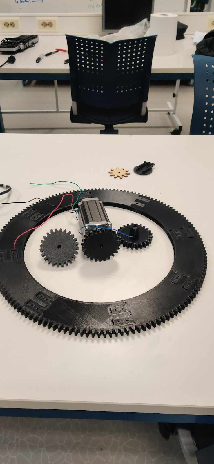
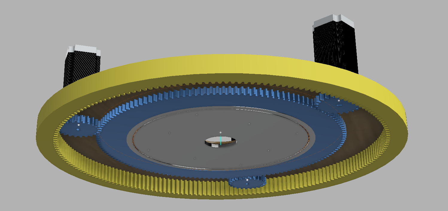
The goal for this week was to produce the parts needed for a working model of the azimuth system. As I had completed most of the design work of the planetary gear system, the parts would now have to be adapted to the production methods available to us; 3D printing and lasercutting of MDF/plywood.

The Teeth Ring of the Sun Gear

The outer race of the slew bearing has now been integrated to the teeth ring of the sun gear. To print the gear, the part  was split into 8 segments with matching protrusions and cavities. 

The obvious choice of manufacture was 3D printing.

As the inner race of the slew bearing would be subject to the most stress due to friction, ABS would be the material of choice. But our group only has access to one individual (Richard Thue) with ABS printing abilities. This would have delayed our production times significantly. Therefore the choice was made to print using PLA.

The parts were printed with a layer height of 0.3mm and 80% infill. 

Total print time: ~29 hours.

The Slew Bearing of the Sun Gear

The outer race of the slew bearing has been integrated with the teeth ring of the sun gear. This leaves the rollers and the inner race of the slew bearing. 

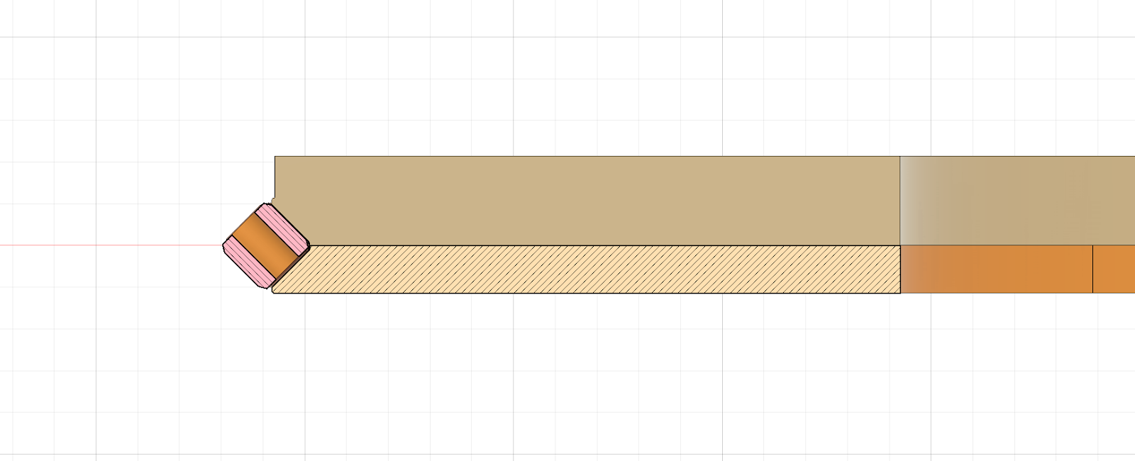
The inner race of the slew bearing consists of a top plate and a bottom plate. Each plate supports one edge of the rollers.

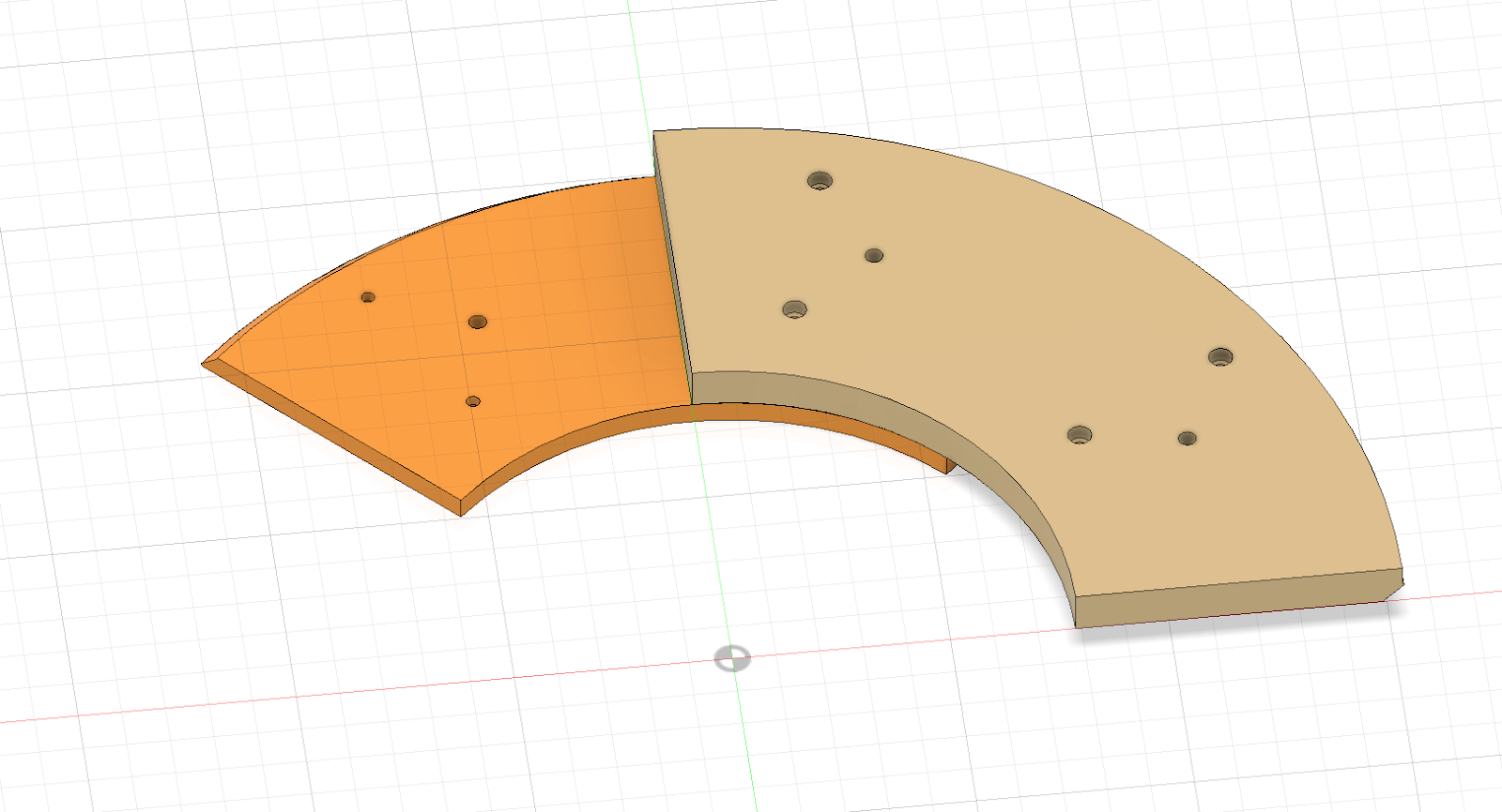
The plates were cut into quarters, where each plate’s cut is 45 degrees offset from the other. This allows us to screw the plates together without need a protrusion/cavity pair.

Again, the material of choice was PLA because of its ease of access.

The plates were printed with 0.35mm layer height at 80% infill. Total print time: ~18 hours.

The Rollers for the Sun Gear Slew Bearing

The bearings (rollers) are 8mm cylinders. These rollers act as bearings in our slew bearing. 

The bearings sit at a 45 degree angle to the normal of the azimuth drive.

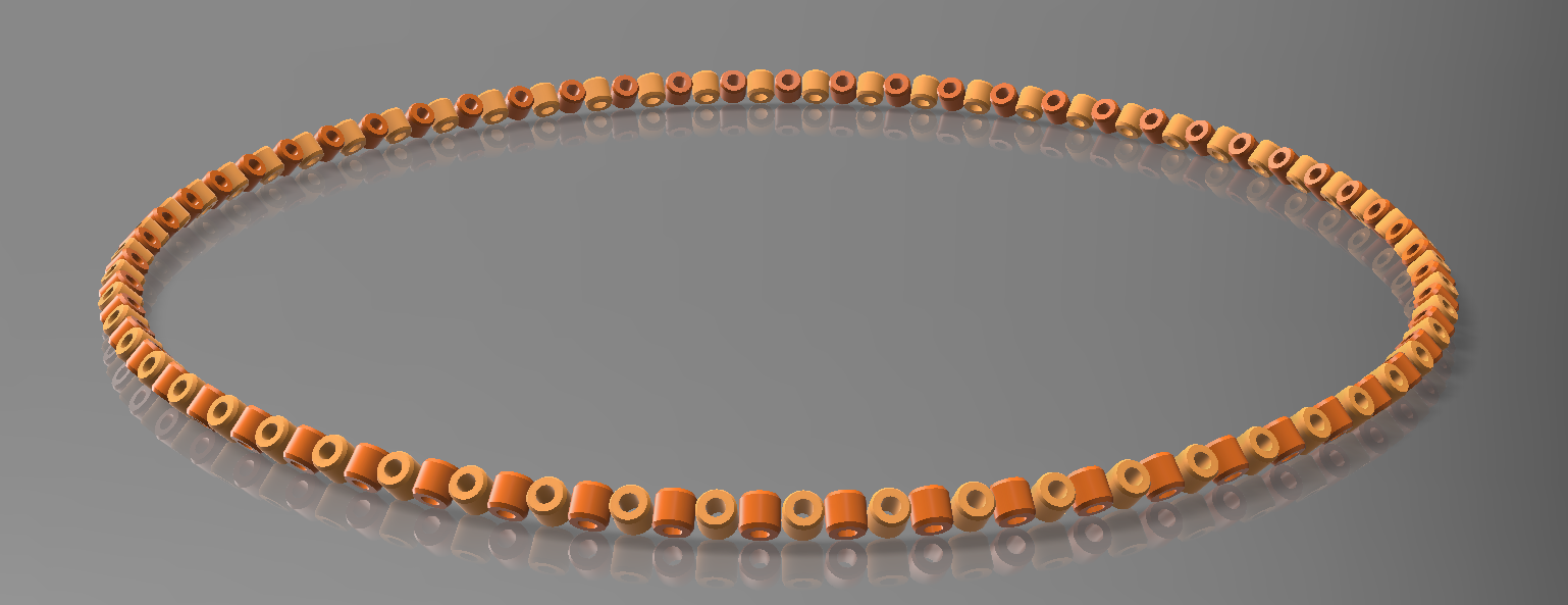
The entire slew bearing consists of 144 roller bearings.

Here our production methods limit our system. The bearings are the main reason and absorbent of friction and thereby heat. Therefore the preferred material would be ABS, as it is more heat resistant; But the timeline of our project prioritized availability.

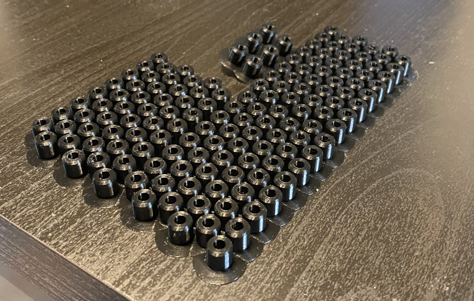
These are 150 rollers printed with PLA at 0.30mm layer height with 80% infill. Total print time: ~9 hours

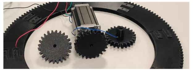
The Planet Gears

Last week we modified 3 Nema 23 stepper motors to feature a D profiled shaft.

The planetary gears were adapted to feature a longer shaft sleeve with a negative D profile in the cross section.

 The longer shaft would give us the flexibility to adjust the proper height of the planet gear in respect to the sun gear

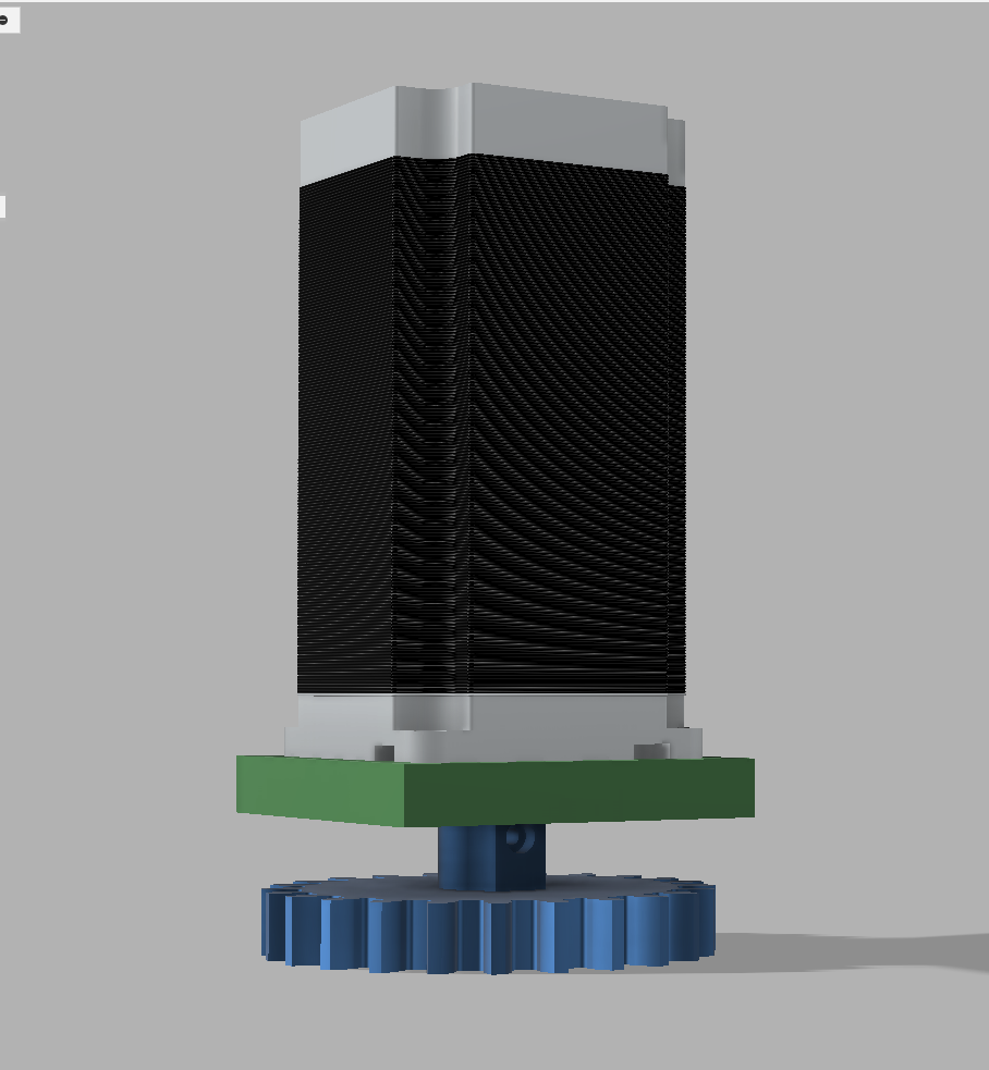
The longer shaft would give us the flexibility to adjust the proper height of the planet gear in respect to the sun gear.

The shaft features recessed holes for M3x6mm screws, but the fit was snug enough that these were obsolete.

The preferred material would have been nylon, as it has the highest abrasion resistance, but our access to nylon-capable printers is even more limited. The next best choice would be ABS, but as mentioned before…

The gears were printed with a 0.35mm layer height at 80% infill. Total print time: ~8 hours.

The Thrust Bearing

The last piece of the azimuth assembly is way of support the inner race of the slew bearing (and thereby plate on which the paintball marker and motors are mounted).

Contrary to the slew bearing where freedom of rotation stems from circumscribed rings, the freedom of rotation would now have to be from parallel plates.

The optimum bearing system is a thrust bearing.

Typically these types of bearing feature either balls or rollers as bearings.

As printing balls is difficult, the choice fell on rollers. 

The rollers are 40mm long, with a diameter of 20mm narrowing down to 15mm. The edges are filleted with a 3.5mm radius.

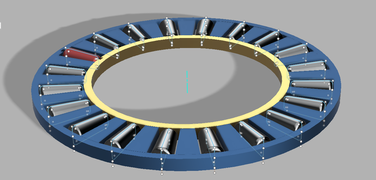
20 of these bearings sit in a cage with an outer diameter of 300mm.

The bearings are supported by 8mm shafts.

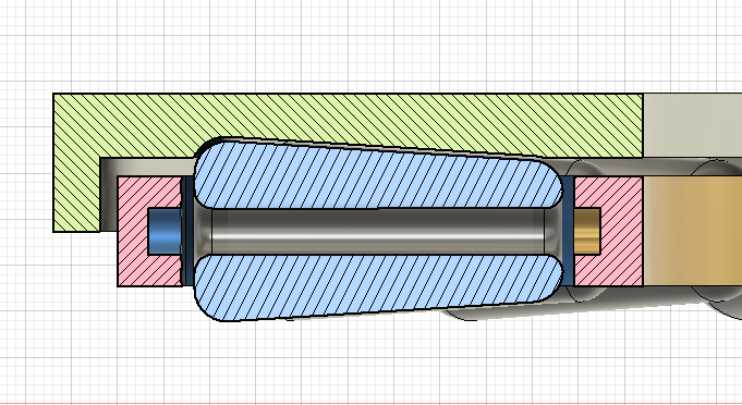
The bearings have 0.5mm clearance from the outer shells. 

As of writing this post, I’m waiting on a 12 hour print of 20 bearings in PLA with 0.30mm layer height at 80% infill. 

Again the material of choice…

Next Week

The goal for next week is to assemble all printed parts, lasercut the outer ring, and make improvements on the design