Demo video:
https://youtu.be/tIBFZ-pgJec
Obtaining access to blood vessels can be difficult. Near-infrared light might be a option since subsurface blood vessels can be visualized in high contrast due to less absorption and scattering in tissue compared to visible light. Instead of using a camera with ingaas detectors, we use a near-infrared sensitivity inexpensive silicon-based detectors. Human perception is limited to the visible spectral range that is defined by the luminous efficiency functions to range between wavelengths of 380 nm and 780 nm. In contrast Si-based sensors in cameras have sensitivities extending to about 1100 nm. Two types of scattering typically exist in the visiblelight and nearinfrared spectral range:
The more intense form of light scattering is Rayleigh scattering, this happens when only the electron clouds are distorted. This is considered an elastic process as no appreciable energy exchange occurs, if energy transfer occurs the process becomes inelastic and is named Raman scattering. This is in general a weak process involving approximately one in every 10^6–10^8 scattered photons.
The first step in developing our analytical method was find and to select the most appropriate analytical technique. This choice will depend primarily on the aspects of the technique such as:
- The principle of analysis
- Error sources
- Limitations or aspects applied during the analysis process
Blood vessels that are used for peripheral venous and arterial access are typically located up to a few millimeters below the skin surface. The blood vessels are embedded in a layer of subcutaneous adipose tissue, at a depth of 1 mm to several millimeters. On top the epidermis 0.1 mm is situated, followed by the dermis 1 mm. The main chromophores in epidermis, dermis and subcutaneous adipose tissue are melanin, blood (mostly hemoglobin, fibrinogen and ALB), proteins and water. In the visible part of the spectrum, melanin and hemoglobin are highly absorptive, counteracting deep tissue penetration. In the NIR part of the spectrum (700–1400 nm), there is much less absorption by melanin and hemoglobin. However above 900 nm absorption of water is increasing, again preventing deep tissue penetration.
It is important that the light generated by the LED is safe for the eye during normal use. Since NIR light is not visible, and therefore a blinking reflex is absent, this also includes longer exposure times. The light generated by the LED is absorbed and can possibly heat the skin.
RAW image processing
There are several available baseline correction methods of the RAW images from the camera approaches with different solutions such as wavelength shifting, first and secondorder derivatives, frequencydomain filtering and simple curve sifting of the broadband variation with a polynomial.
Partial least squares regression is a commonly used quantitative multivariate statistical tool that allows for the analysis of data with strong correlations and with noise to model a response variable when there are a large number of predictor variables[1]. Partial least squares regression can also handle data sets with more variables than samples. In analysis of biological samples, usually the most important spectral signatures are the fingerprinting peaks in the images that represent the biochemical region of the image. Binary bar-codes calculated from signs of second derivatives can be used to further remove the redundant information in the intensity fluctuation due to all the sources of intensity, this can be unexpected reflections in the image. We also lock at different methods to remove outlier images, image outlier diagnosis is a very important step to identify system faults in building reliable image sample set. Proper procedures for elimination of outliers are valuable tools for improving the quality of spectral fitting from averagedpixels. Another pre-processing method we looked at is normalization, which intensity values are rescaled for consistency. Normalizationis frequently used as a pre-processing step in preparing reference images for a qualitative identification library[2].
[1] Randall D. Tobias, SAS Institute Inc., Cary, NC, An Introduction to Partial Least Squares Regression
[2] Bocklitz, T., A. Walter, et al. (2011). How to pre-process Raman spectra for reliable and
stable models? Analytica Chimica Acta 704, 47-56.
We started by trying to use the wiringpi library in python to control the movement of the servos, we soon found a few problems by doing it this way. We got a lot of gitters on the servos, so they would start twitching and move at very irregular speeds. One time it might move 300 steps and the next time it would move 150. We needed way better precision and reliability for the Angstanjagende Robot Naald.
After a little research I figured that the process that was creating the output signal from the raspberry pi were getting interrupted by other processes from the os and other applications on the raspberry pi. And since the servos are dependent on getting the correct length pulse at the correct time to move in the correct direction, this made the servo sometimes move backwards for a few steps when it was supposed to go forwards and the other way around. To fix this I increased the priority of the program to max (nice -20) and isolated the program to run on a single core or the raspberry pi, not allowing any other processes to use that core while the program was running (taskset -c 3). 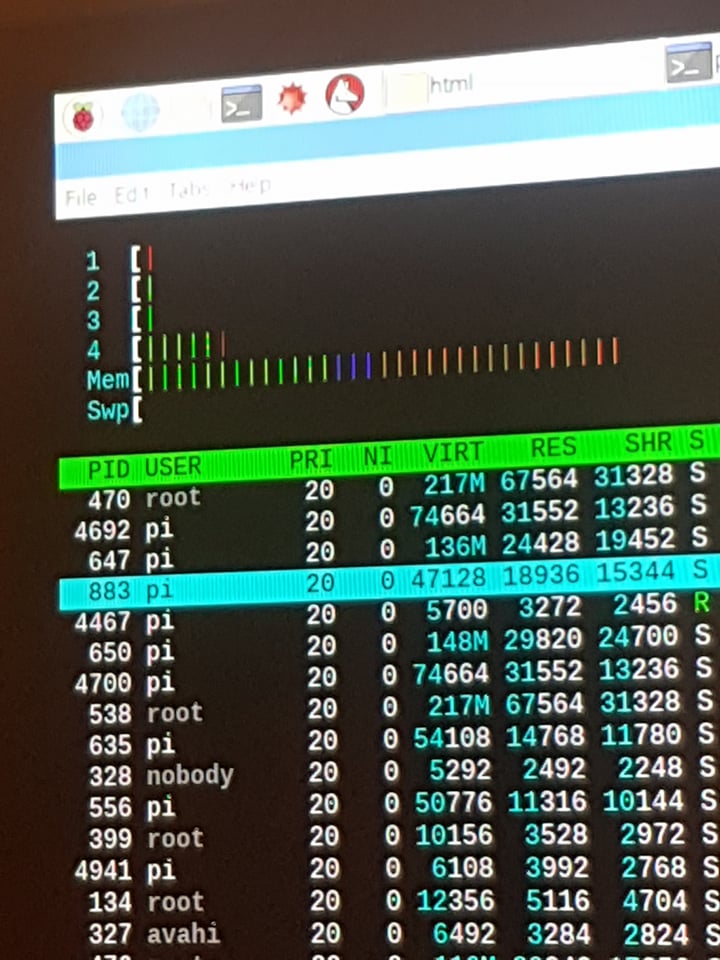
Checking the cpu usage while testing the python program.
Since the raspberry pi has a quadcore processor and there were no other heavy programs running the raspberry pi didn’t have any problems running on core 1, 2 and 3 for regular processes and core 4 for the raspberry pi program. This gave us a much more stable result. The precision was still not good enough because the servo control on wiringpi library for python didn’t allow controlling exactly how many steps the servo moved, so it was controlled by time instead. The sleep function in python was only precise down to milliseconds and to move the servo forwards it needed pulses of 1,3ms and backwards it needed 1,7ms.

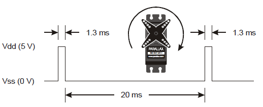
Sample timing diagram for a centered servo.
The Parallax Continuous Rotation Servo is controlled through pulse width modulation. Rotational speed and direction are determined by the duration of a high pulse, in the 1.3 -1.7 ms range. In order for smooth rotation, the servo needs a 20 ms pause between pulses.
Clockwise direction.
As the length of the pulse decreases from 1.5 ms, the servo will gradually rotate faster in the clockwise direction.
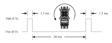
Counter-clockwise direction
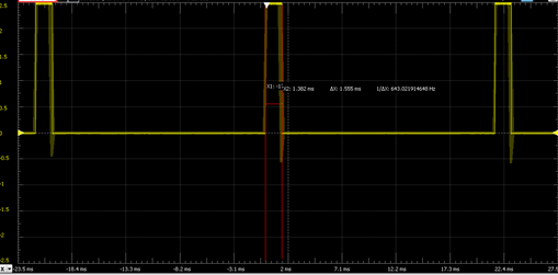
As the length of the pulse increases from 1.5 ms, the servo will gradually rotate faster in the counter-clockwise direction. We measured the pulse width and time between each pulse and found that the time between each servo was a lot sorter then what it was supposed to with ca 4ms between each pulse rather than the recommended 20ms.
Clockwise pulse width of 1,5ms
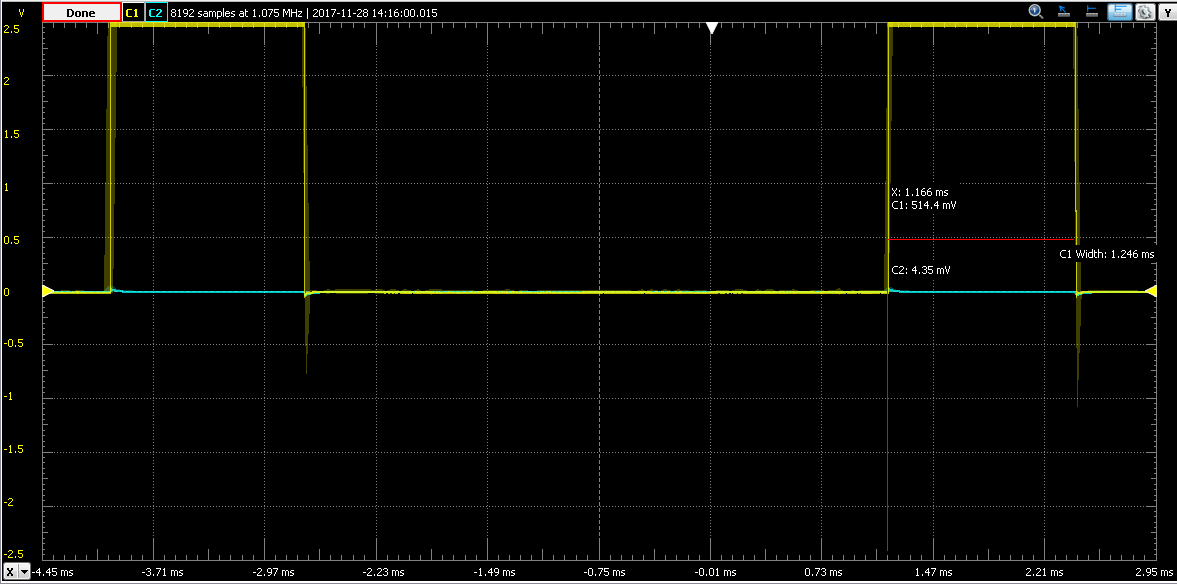
Counter clockwise pulse width: 1,16ms
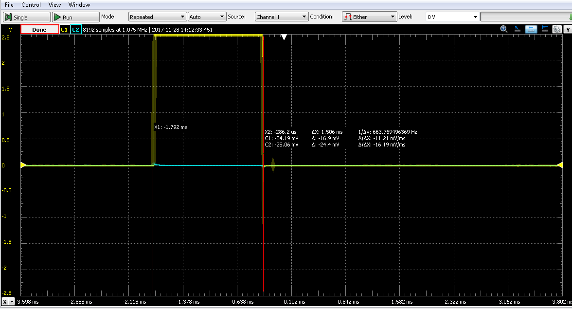
We experienced issues with the servo motor as we noticed that it did not respond to our program commands. We decided to use an oscilloskop from the program: Digilent WaveForm, to take measurements to see the output from the raspberry Pi. Then we noticed that the pulse width was incorrect.
Because of this we threw away the idea of using python and made a new script in c, since c is a lower level language. This gives us a lot more control by manually setting the output pins for the raspberry pi. C also has the usleep function that can sleep in microseconds instead. Making it possible to give the servo the correct pulses and control the exact number of steps a servo moves. To decide how far the servo was going to move in the x and y axis we have a x and y coordinate that we get from the matlab script that analyze the picture.
When we tested the servos on the Angstanjagende Robot Naald we saw that the servos moved further backwards than forwards when it was set to move the exactly same distance forwards and backwards. We measured the offset per centimeter in each direction and added it to the x and y axis. Now the servo moves the exact same distance forwards and backwards, so it always end up on the same spot as it started after running the entire program.
Now that the servos were moving the way they should we made a bash script to make the different scripts run in the correct order (smartSystems.sh). First taking a picture with the camera attached to the raspberry pi, then running the matlab script to analyze the picture and figure out the coordinates and then running the servo control program to move the servos and make the mark where the blood vessel in the arm is. We also made the bashscript run at startup, so we don’t need the keyboard, screen and mouse connected to the raspberry pi just the power. There were a few different ways of setting up the autostart. We figured writing the startup.sh script in the /home/pi/ folder together with the smartSystems.sh script and adding the shortcut.desktop script to the /home/pi/.config/autostart folder. This makes the smartSystems.sh script run as soon as the rest of the raspberry pi has started up, and is the solution that worked the best for us.
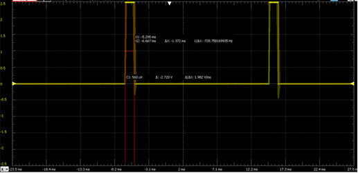
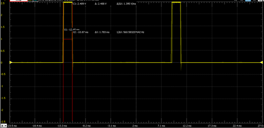
We wanted to check the pulse width again with the scope, and we verified that the correct pulse width was within servo specifications, as explained before.
Centered servo, pulse width: 1,5ms
Clockwise direction, pulse width: 1,3 ms
Counter-clockwise direction, pulse width: 1,7ms