Bram van den Nieuwendijk
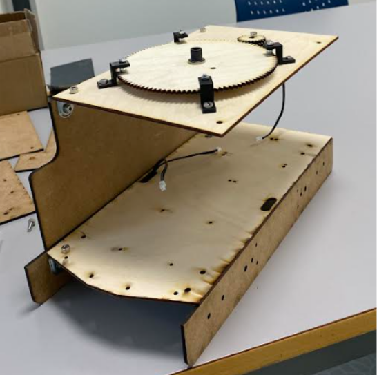
This week, I began by 3D printing several parts and doing some laser cutting to continue building the prototype. The bottom section of the prototype is now ready for testing as soon as the wheels (currently being 3D printed) are completed. The rotation mechanism for the top part in the x-direction is also ready to be tested. Additionally, I sent more parts to Richard for 3D printing so I can start assembling the y-direction rotation mechanism. Hopefully, these parts will be ready next week, allowing me to begin testing the full prototype. Once the prototype performs successfully, I plan to replace the laser-cut components with 3D-printed ones.
Sulaf Bozomqita – Week 11: Acceleration Logic & Smarter Avoidance
This week I focused on improving the obstacle detection system by adding acceleration/deceleration control and refining the avoidance maneuvers. As usual, I worked independently for this segment. Now, the reason decided to implement the acceleration and deacceleration was because I know this would make a smoother and safer navigation for the robot.
Last week, I successfully integrated my module with Åsmund’s motion control interface by making a MotionControl class too, to test and validate my module with the navigation module in reality, using a lookup table for PWM values. However, the speed changes were very abrupt in my opinion, and that would translate onto the robot as less smooth navigation. In addition, the avoidance was based on fixed delays. Thus, my goal this week was to make transitions more realistic and dynamic.
Updates made this week with the code:
I added acceleration and deceleration values for a smoother transition during navigation. I implemented a gradual speed changes:
- When resuming navigation, the speed ramps up smoothly instead of jumping to full speed (no more sudden movements).
- When stopping for an obstacle, the PWM decreases gradually and not suddenly (you can see that in the colsole, the progression of slowing up and down while navigating around an obstacle).
- Used timestamps and formulas for acceleration:
v=v0+a⋅t (the physics formula for speed). And for the stopping distance: s=v2/2a
Dynamic Avoidance Maneuvers:
I also made a dynamic avoidance maneuverability this week, so that when it backs up, it does so until the front sensor reads a safe distance (instead of having a fixed time).
The new updated code also turns left or right based on dynamical sensor readings. Then, to maneuver around an obstacle, it resumes forward with gradual acceleration for smoother recovery.
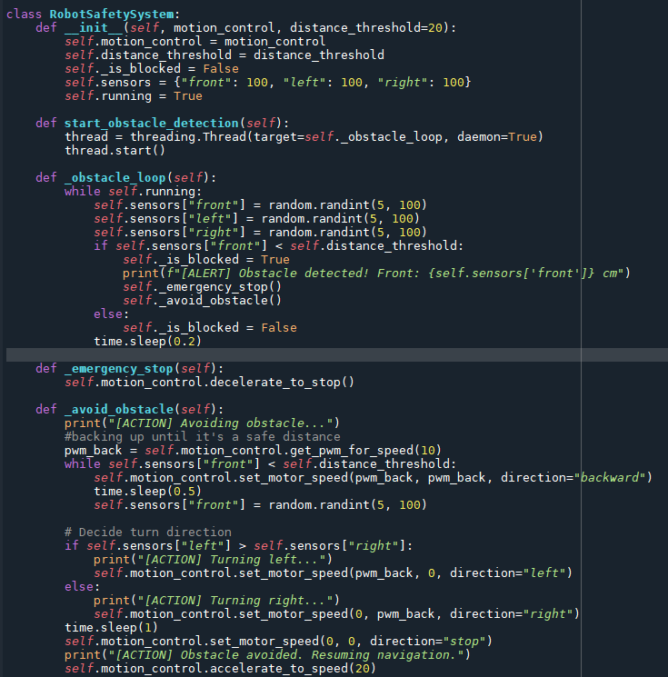
Code of what I updated and improved on this week (as stated above):
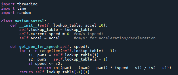
This shows the speed used, utilizing the PWM for speed as well.
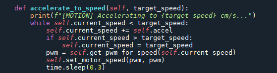
The acceleration function for smoother transition I made this week:
The deacceleration function for stopping I made this week:
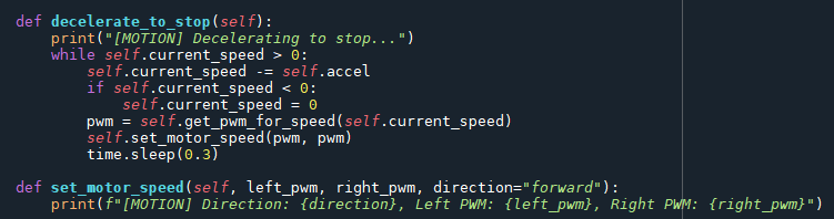
The rest of the code:
Testing Setup:
Hardware is still unavailable, so I continued using simulated sensor readings and PWM outputs. But again, it does not affect any of my code.:
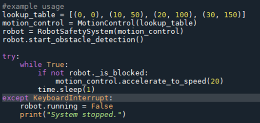
Output:
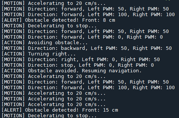
The console logs show the gradual acceleration steps when resuming speed, dynamic avoidance decisions based on sensor data, and a smooth PWM transitions during emergency stops.
Åsmund Wigen Thygesen
This week I was going to set up our compass with the raspberry pi. We were planning on using an LSM303DLHC accelerometer and compass IC, but it was unfortunately forgotten about when we sent in our list of components to buy and now it’s too late to get it. So instead we’re going to use a microbit for its compass.
The plan was to have the microbit act as a slave I2C device, just forward it’s own compass data to the master when requested. However, turns out the microbit I2C chip is hardwired to be a master, the raspberry pi can be configured as a slave device and it should technically work to use a setup like that to achieve what we want, but initially I dismissed that thought and considered other options and found a different solution.
The other data busses are also unavailable since our PCB which interfaces with the raspberry pi has already been made and the pins are occupied. However, the microbit v1.5 uses a similar compass IC to what we were planning on using and the I2C bus that the chip is connected to is the same as the one that is exposed to the edge connector (this is not the case for microbit v2+). This means I should be able to communicate directly with the compass from the raspberry pi, so long as those pins are set as floating in the microbit processor.
The IC is an LSM303AGR, which i found out is not supported by the library I was planning on using…and I can’t seem to find an appropriate library for it. So I guess this is a good opportunity to learn more about the I2C protocol.
After some reading I was able to read the magnometer registers on the chip using the smbus library, which does writing and reading of registers over I2C for you. So now I was able to read the data, but it was not calibrated and could not be used to accurately tell the angle of the vehicle.
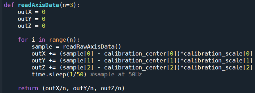
At startup the A and C config registers are set, we mostly just use default values, except the A register, where we set the sample rate to 50Hz

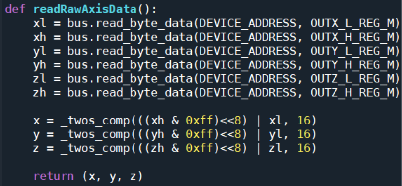
Then we just need to read the output registers and combine the bytes for each component, this code is essentially a copy from a forum post and am realizing they also do a twos compliment conversion, which I don’t think is necessary, but I’ll have to look more into that next week.
So I needed to do some calibration, initially I tried a simple calibration technique that I found in the same forum I used to base my initial code on, but it turned out to not really help much, not enough for our purposes at least. So I moved on to reading through the microbit source code to find their drivers and calibration code.
When the only magnetic field present is that of the earth, a perfect magnometer should in theory produce a constant signal magnitude across the x, y and z axes. So that is what the microbit calibration code tries to correct to and is the approach I took as well.
The calibration has 3 steps
First I obviously need to sample some datapoints to use for the calibration. Here I found that doing 80 reads over 10 seconds works well, and as the data is sampled I tilt the microbit smoothly around trying to get a somewhat even coverage of datapoints across our imaginary sphere.
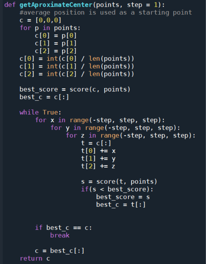
Then we need to get the centre of the sphere, which importantly is different from the centre of the datapoints, since the datapoints can be more densly populated on one side of the sphere, but we need the centre of the sphere. We start by taking the average and use that as a starting point, then we use a hill climb algorithm to iterate towards the centre, this is the was microbit does it, but I first decided I wanted to try implementing a gradient descent algorithm which should be able to do it faster and more elegantly. I did kinda succeed, but my implementation ended up not being faster and generally being more inconsistent, so I fell back on basically just copying what microbit did and ended up with this.
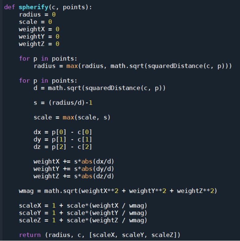
From there we essentially find the point furthest from our centre and call the distance from it to the centre our radius. Then we calculate the scale factor needed for each point to be on the sphere, then add the x, y and z components to a “scale weight” vector, which we normalize and multiply with the largest scale factor to get our final scale vector.
To apply the calibration we simply subtract the centre position from the reading and multiply by the scale vector. I also take a couple readings and average them for consistency.
Rick Embregts
This week most components for the PCB’s have arrived. Now I have to wait for the PCB’s themself to arrive to begin the assembling process. While picking up the pcb components I noticed that the motor’s weren’t with the package. Due to miscommunication, it was believed that we didn’t need the motors anymore. This is a big setback since we need to get the vehicle operational as soon as possible.
Since I didn’t know when the pcb’s would arrive, I started working on a backup plan for the electrical system. In this backup plan the entire system gets powered by a PSU from school. In this backup plan the motorcontroller wil be borrowed from school and the relay for the spray motor will be seperate from the motor controller. Next week the schematic for the backup plan well be ready.