Hello and welcome back!👋
This week marked another milestone for the Hydrawlics team. We completed our midterm presentation, and it went really well! With Sprint 3 now behind us, we’re starting to see more and more of the arm come to life; both physically and digitally.
Here’s what the team has been working on this week 👇
Fredrik:
This week we completed sprint 3. From the mechanical side, our goal was to have a prototype of the arm structure. I was responsible for the arm segments, joints and end effector prototype.
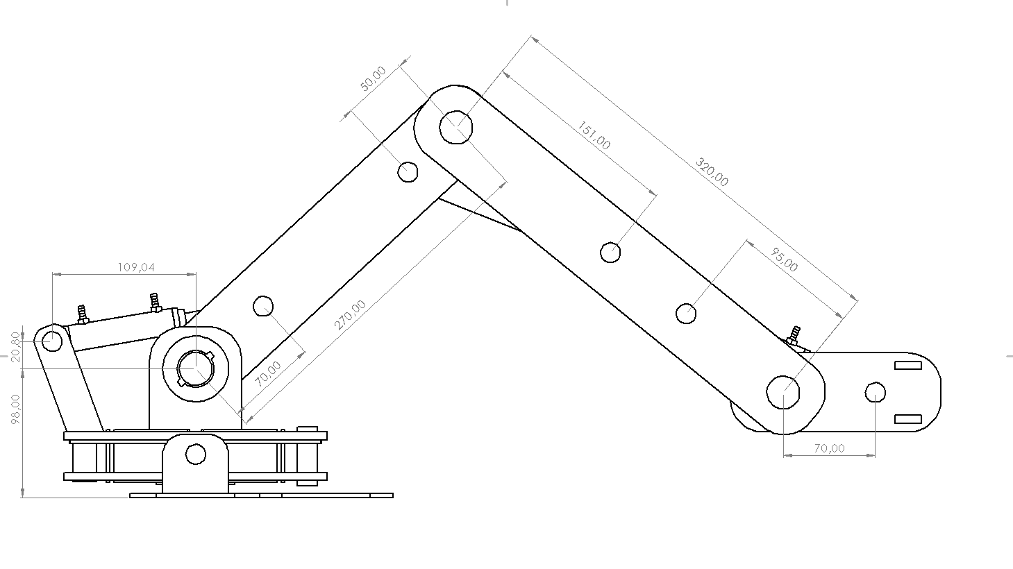
To achieve this, the layout first needed to be defined. I have played around with different arm segment lengths and cylinder placements for a couple of weeks now, to see how it would affect the drawing area and shape of the arm. The layout I landed on gives a large drawing area, but might demand too much from the hydraulic system. This will need to be tested when this is possible. The tentative layout is shown in the picture below. (The picture is for visualizing distances only, and is not a technical drawing)
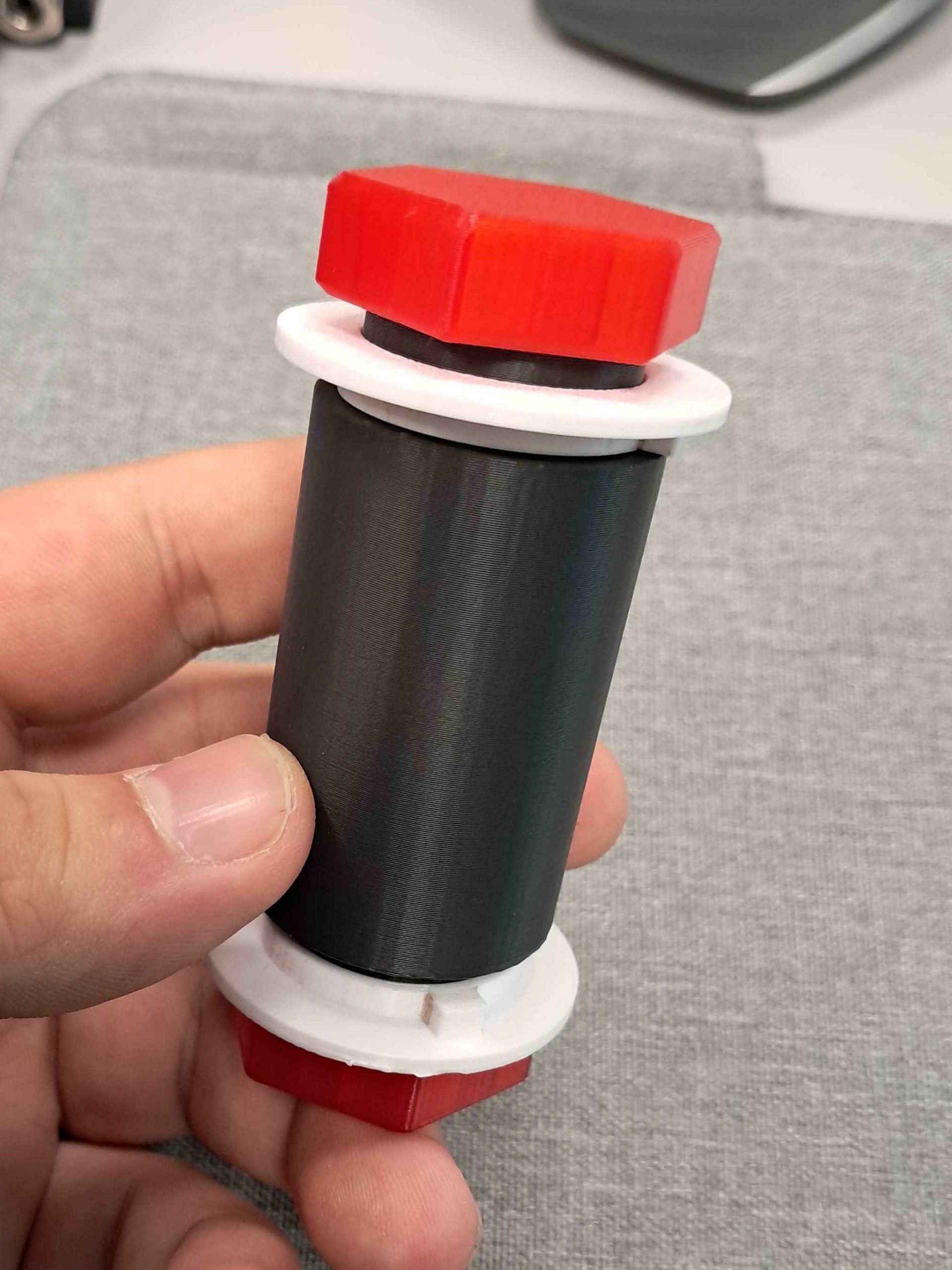
Seeing as what we are currently developing is a prototype, I think it would be beneficial to design it with the ability to be disassembled. Earlier in this course, while working on the hydraulic cylinder, I fastened parts to each other by pressfit, without the ability to remove them again. This turned out to be a nuisance. Therefor, I wanted another non permanent way to fasten components, and turned to 3d-printed bolts. This is something I have wanted to learn how to do for a long time, and thought now would be the perfect opportunity. I watched some YouTube videos and tested for myself, and it worked great. It opened the door for secure fastening, with easy assembly and disassembly.
While the arm segments would be made out of lasercut material, I decided that the joint should be made out of 3d-printed components. In the design, the two lasercut plates are separated with a bushing in between to prevent them from rubbing against each other. That would lead to a lot of friction, and variable friction area based on the position of the segments. PLA has relatively low friction against PLA, so I design the bushing and joint shaft accordingly. Finally, a bolt on each side to hold everything in place. I choose inner threads and a bolt over outer threads and a nut because I think it would be easier to print, and easier to assemble.
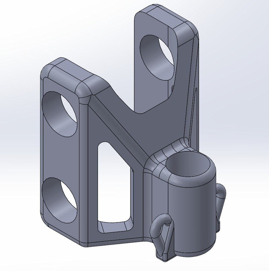
I have included images of the 3d-model of the joint below. I included notches in the interface with the lasercut plates, to lock their rotation to each joint component. Now the inner plate rotates with the bushing, and the outer plate rotates with the joint shaft. This ensures that all rotation takes place between the PLA components, and not the lasercut plates. Locking the outer plate to the joint shaft also ensures that the bolt’s rotation is always the same as the plate directly below it, greatly reducing the risk of it loosening during operation.
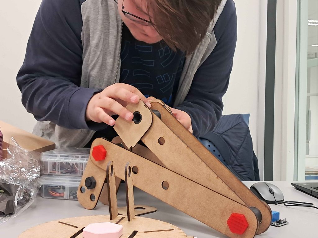
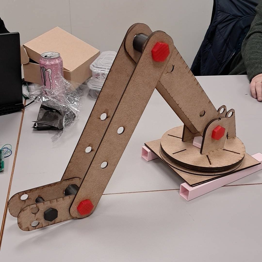
The arm segments was lasercut at school from mdf plates. After a couple of mishaps, the results looked promising. The plates seemed strong enough, and it was really cool to see the true scale of the arm segments. The printed parts fit together with the lasercut parts perfectly, and the joint system worked as intended. After successfully combining my design of the arm segments with Erlings design of the base, the arm structure was complete. This meant that we now need to finish designing and start implementing the hydraulic system, before we can run our first real tests.
I didn’t have the time to include the end effector prototype in the physical model this week, but the 3d-model is shown below. It fits only one type of marker, but is fastened with bolts to enable easy swap for other designs. This design holds the marker down to the holder by elastic rubber band, which should at least be good enough for a prototype.
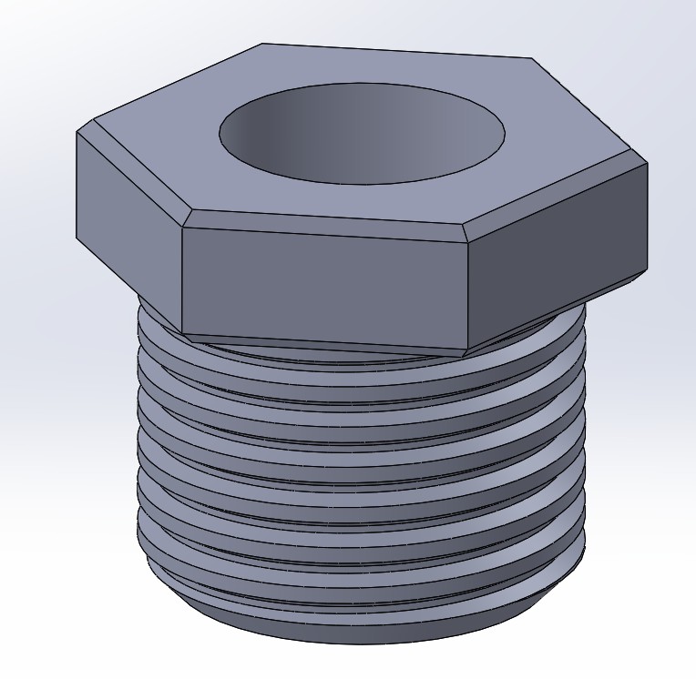
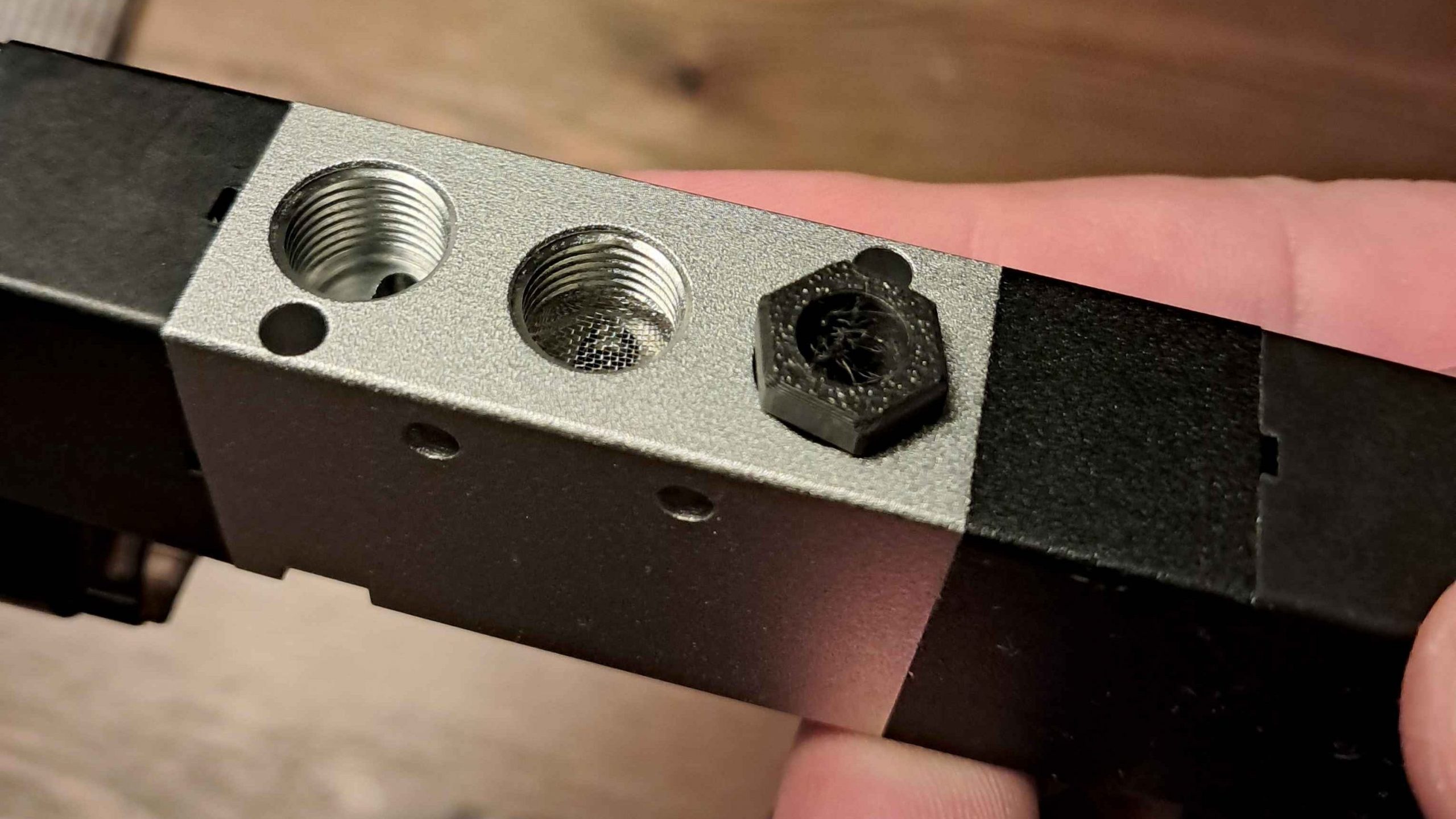
The valves we ordered arrived this week, and need some attachment module for our tubes. Me and Erling was thinking of using push-in fittings, but realized this would cost around 500-600 NOK. We are therefor looking into alternatives. The valve has 1/8 inch taper pipe threads, so I am looking into 3d-printing threads to match this. Using online resources to calculate the diameter and thread pitch, I managed to print an attachment that fit the valve surprisingly well. Safe to say I have learned a lot about threads this week. I think making sure it does not leak will be a challenge moving forward, but this is a good start.
Lisa:
After a week away, I’m finally back in full swing and ready to continue developing.
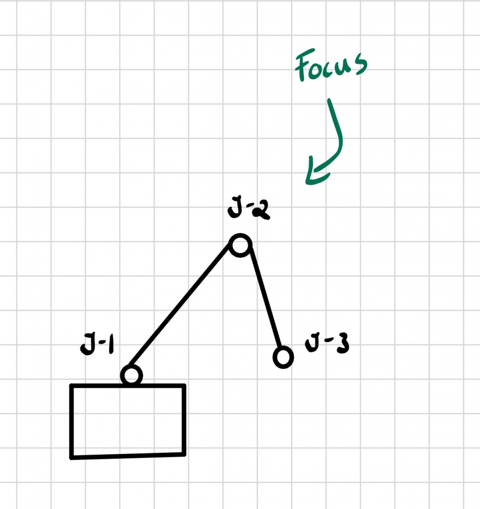
This week, we successfully held our midterm presentation, which I think went really well! After the presentation, I continued focusing on my task, which was to extrapolate the angle of the potentiometer used to measure the rotation of one of our hydraulic joints (J-2), as shown in the figure below.
Understanding the challenge
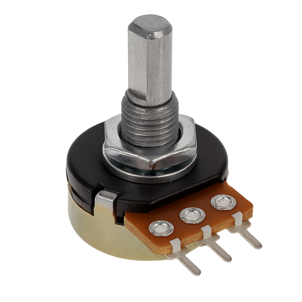
A potentiometer provides an analog voltage signal that varies as it rotates. The Arduino reads this signal as a number between 0 and 1023, this is also known as the ADC (Analog-to-Digital Conversion) value. However, this raw number doesn’t directly tell us the joint’s angle in degrees. To make the data useful, it had to be converted into a physical angle that matches the actual movement of the joint.
Establishing the ADC angle
To obtain specific and accurate angle values from the potentiometer, I first needed to calibrate the system. A potentiometer only gives raw analog readings (0–1023), so to make these meaningful, I had to map them to the actual physical angles of the joint.
- Turned the potentiometer to its minimum position and recorded the lowest ADC value (a_min).
- Rotated it to the maximum position and recorded the highest ADC value (a_max).
From simulations, we know that J-2 moves between 54° (min) and 98.2° (max).
With these two known points, we can describe a linear relationship between ADC readings (a) and the corresponding angle (φ):
φ=m⋅a+b
where;
m: is the slope (degrees per ADC step)
b: is the offset ensuring the output starts at the correct base angle.
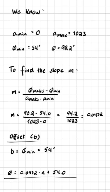
This means that each ADC step corresponds to roughly 0.043° of rotation.
Implementation
Once calibrated, I implemented the formula in code and connected a LCD display to visualize the live angle values. The screen now shows the current angle in degrees, along with a progress bar that moves as the joint rotates. When the potentiometer reaches its limits, the display clearly indicates “MIN” or “MAX”.
This small addition turned out to be incredibly useful, and it gave a nice, interactive feel to the setup.
Relay testing
With the potentiometer system up and running, I looked attesting the 8-channel relay module, and the main goal was simply to confirm that everything worked as expected. The relays will later be used to control the pumps and valves in our hydraulic system, but for now, I focused on getting the basic setup running.
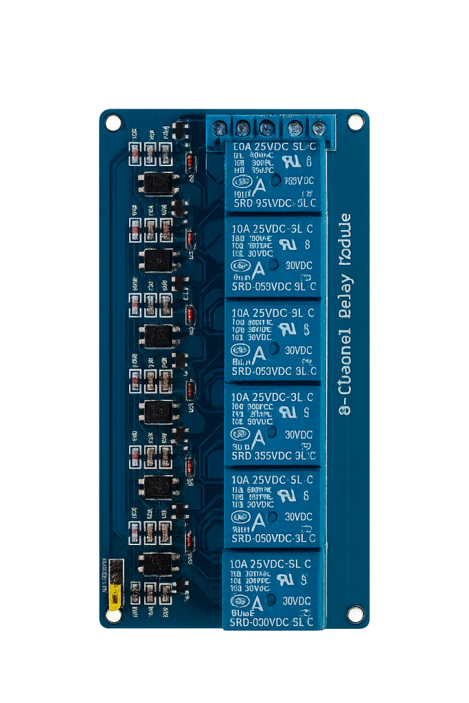
After identifying the control pins (IN1–IN8), power, and logic connections, I uploaded a short test sketch to switch each relay on and off. All channels responded correctly, and the distinct clicking sound confirmed that the module was functioning properly.
To make it a bit more fun, I also added a simple pattern where the relays activated one after another in quick succession
Overall, everything worked as intended! Everything from reading stable angle values in the potentiometer to controlling all eight relays in sequence.
Syver:
Hello! Last week we mentioned that much of the planning and design on the software side was done. We needed somewhere to test the software before we could integrate with the hardware. Therefore, the next natural step was to enter The Matrix and test our arm there. This is what I’ve done this week.
To build the simulation, I first needed the mechanical specifications. Our mechanical engineers have defined a preliminary layout for each joint, arm segment and piston; fully defining the domain of freedom. See Fredrik’s part for the diagram. Using this, I started throwing together its ugly twin in Unity.
This was new territory for me. I haven’t really had any experience in Unity or C# before, so some time went into learning how it works, with AI as my tutor and assistant. After a while, I got the hang of the scripting basics, and implementing code went a lot smoother. I grew to enjoy the way C# interfaces with game objects through tooltips on public variables, which made it really simple to treat each joint as an instance of a class, and assign the HydraulicJoint script to each of the joints.
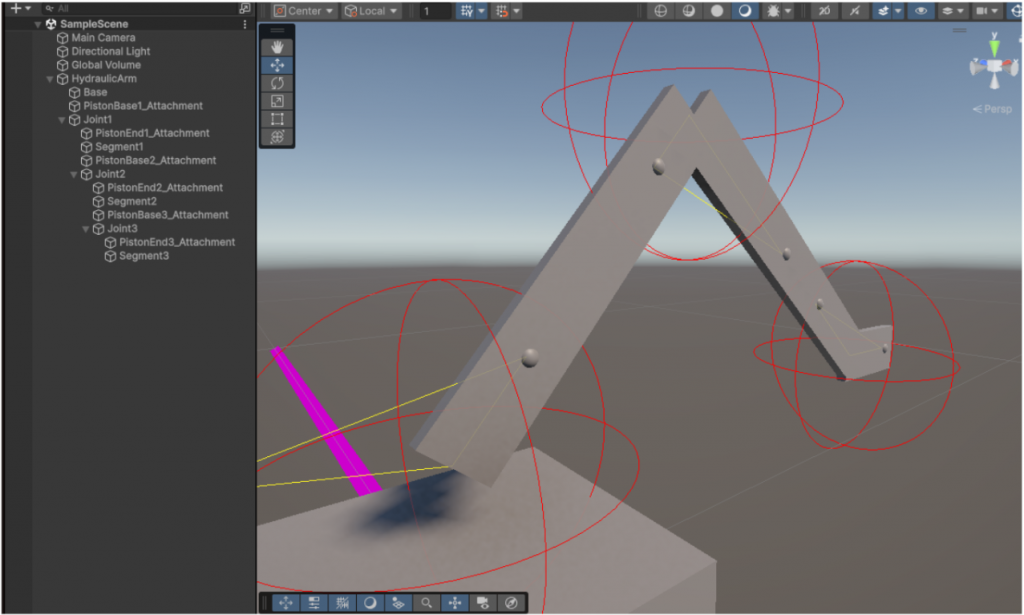
The hierarchy of the Unity objects makes the movement pretty intuitive. Being a child of an object means that you rotate with it. In this case, if Joint1 rotates, all its child segments and joints will rotate with it, propagating movement outwards. This is perfect for structuring our arm segments.
With the game objects in place, we need to rotate the joints (and thus their children) to a given target orientation. Each Joint object, seen in the object tree on the left, has its own HydraulicJoint.cs script attached handling rotation. A simple task at surface level, but we wanted the simulation to include as many of the real-world elements as possible. This includes the binary valve switching and piston placements, making the implementation a tad bit harder.
First, we need target angles for each joint. Accurately modeling piston movement is challenging because the pump’s flow rate is hard to predict. Therefore, each joint is using potentiometers for angle feedback with PID-control for correction. This isn’t ideal for quickly following predefined values, but we can mitigate inconsistencies through positional “checkpoints” for each vertex/command, as well as lowering the speed or flow rate. PID should be enough for our project requirements, though other control methods might be worth checking out if we have time.
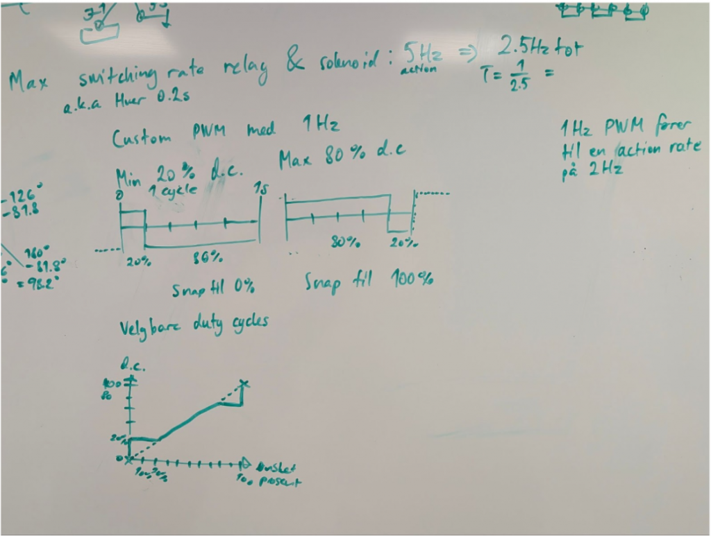
Using these outputs, we can convert the corrective values into duty cycles. These are fed into a valve simulator, multiplying the piston direction with the guesstimated piston velocity if within the PWMs on-state. This would’ve been fairly straightforward if it weren’t for the mechanical 5Hz action frequency limit of both the relays and the solenoids. This means that the smallest interval between two state toggles is 0.2s. The maths can be seen below, but in summary, with a 1Hz PWM frequency, we need to clamp the duty cycle to 0%, 20%-80%, 100% as seen in the bottommost graph. This will somewhat degrade the resolution in movement, but we already knew this would be a limitation to some degree.
Once these elements were implemented, the virtual arm was moving as expected! Each joint’s target angle can be manipulated with the arrow keys. Having this interactive model made it much easier to visualize the different piston movements, including speed, stability and the performance of the PID-controller. See the arm in action!:
The next step will be to add a virtual whiteboard where the arm can draw. After that’s landed, we’ll implement the reverse kinematics, which will be much easier with this virtual arm, keeping our software bugs from having any real world consequences (yet).
This Unity project is our third and final project repository, available at https://github.com/7RST1/hydrawlics-sim-unity. The scripts discussed in this blog post are Scripts/HydraulicJoint.cs and Scripts/HydraulicArmController.cs.
Emory:
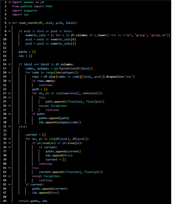
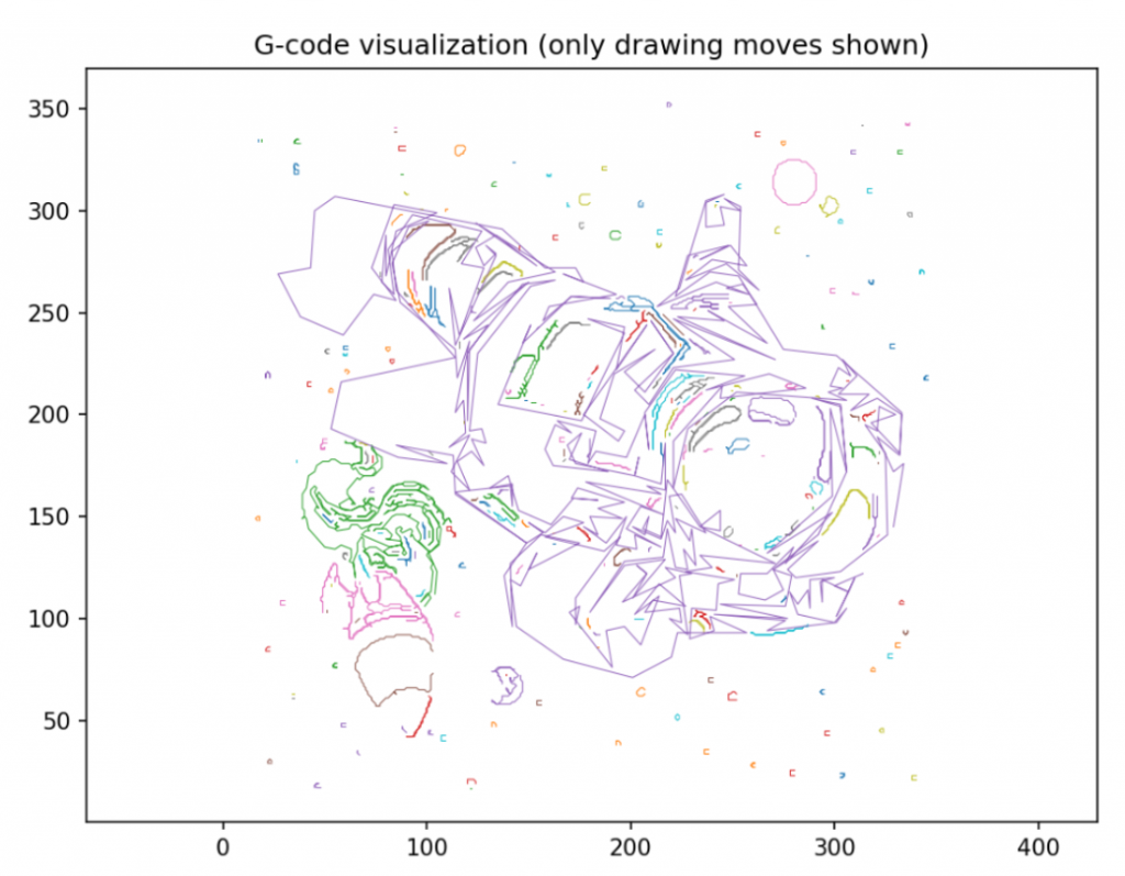
This week, I continued working on the code to convert coordinates into G-code. The code starts with read_coords, which reads the coordinates from the csv file that contains the polygon IDs and the x, y coordinates for them. The longest part of this part of the code is to make sure that each polygons get saved separately and then saved into ID.
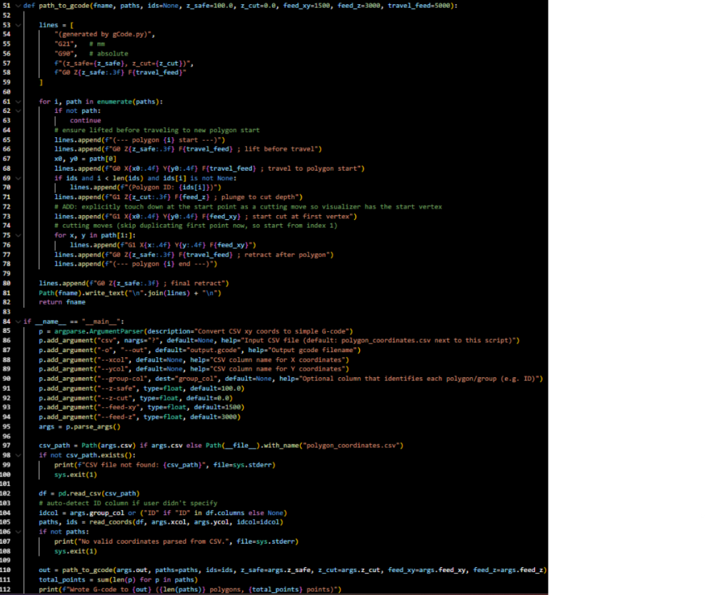
Then path_to_gcode converts all the coordinates into g-code commands. It starts with setting the header and then getting to the starting point. It got a set z_safe, which is the safe height it starts at. After each polygon, it draws it goes back to the start point G0, it also goes back to G0 when it’s drawn.
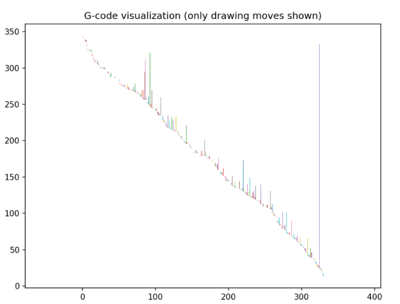
I had a problem in the beginning with the output of the g-code coordinates, where they looked like this:
I solved this by realising the ID was being put into the x coordinates and the y into x. So by fixing this like the code above, the output looks correct. So now we get the g-code like the image below from the code.
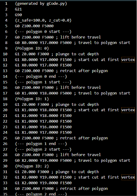
This works in making sure the image is what we want it to be now in g-code, which is better for the arm to use for movements.
I removed the minimize_path function for now, as it works fine for what we need it at the moment, and might add it later if we feel there’s a need to optimise the drawing pattern.
Erling:
The week started with Midway presentation. Which to me seemed to go pretty well.
This week we continued the development of our system. This week was the last week of Sprint 3 for us, where our goal was to have a “functional” prototype with 2 or 3 Degrees of Freedom.
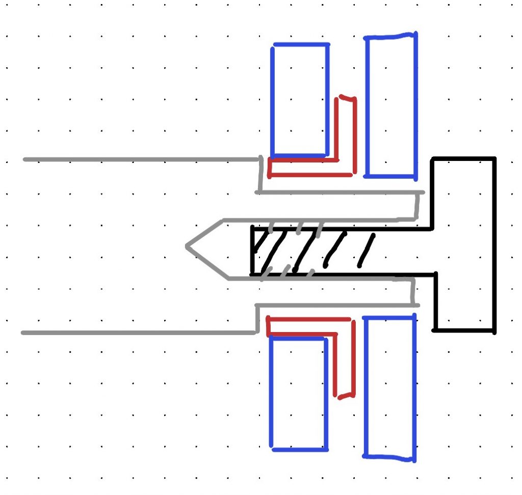
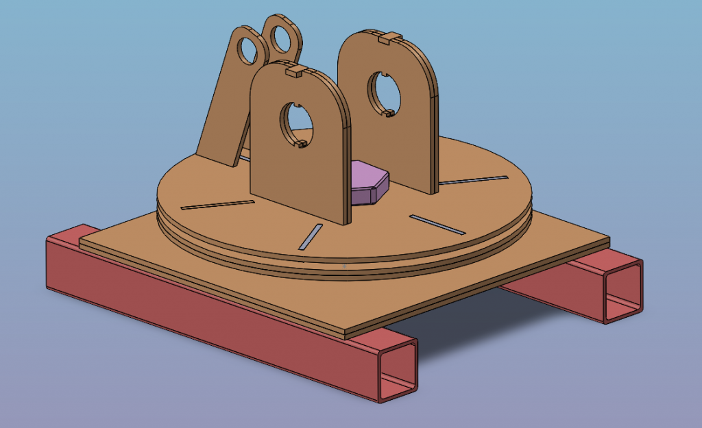
I took the preliminary design of the arm by Fredrik a few weeks ago, and did the detail design for the base of the arm so that it will function as we want it. In the image below we see the Azimuth axis of the arm at this stage of development. We are utilizing axial bearings in order to constrain the 5 other degrees of freedom in this joint of the arm. This design was chosen because it would be cheap for us to produce, and that we could realize it relatively quickly using 3D-Prints and laser cutting using the equipment at school.
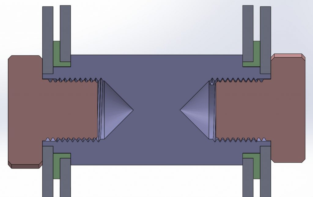
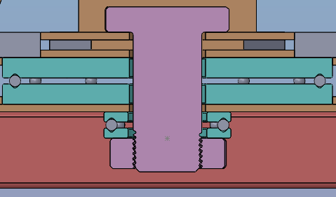
Below we see a crosssection of the base of the arm. Here the Axial bearings are clearly visible in blue. In reality these aren’t actually purely Axial bearings, as the rolling elements are rolling in bearing races that slope. These are really comination bearings, and they serve both functions in this design. As the bolt in pink has a few millimeters of clearance to the holes, the bearing serves as the axis locator for the azimuth axis.
I realized that we need two bearings for this to work in order for the bolt to not loosen under rotary movement of the base. This would result in loss of preload on the bearings, and ultimately lead to the base falling apart.
As this is important does not happen, i added a bearing between the stationary base and the nut, so that the whole bolt may turn with the rotary joint.
For clarification; the large upper bearing is responsible for allowing a single rotary degree of freedom in the base of the arm, and the smaller lower bearing is there to allow the nut to rotate with the upper portion of the base in order to maintain preload on the larger bearing.
The rolling elements are intended to be Airsoft BB pellets as they are sufficiently round, and hard enough for this application.
At the same time, the hydraulic system development continues. We have recieved the valves that we ordered. Now the focus for the hydraulic system is getting all the miscellaneous part that we need in order to make the whole system work. That means that we need more PVC tube to fit our water pump, push to connect fittings and distribution manifolds for the valves. I plan to purchase the needed lenght of tube in the coming week. The push to connect fittings are another such item that will cost us more than 500kr if we were to purchase them, so we are looking into making our own solution for the project. more on that either in Fredrik’s part, or in the next blog post.
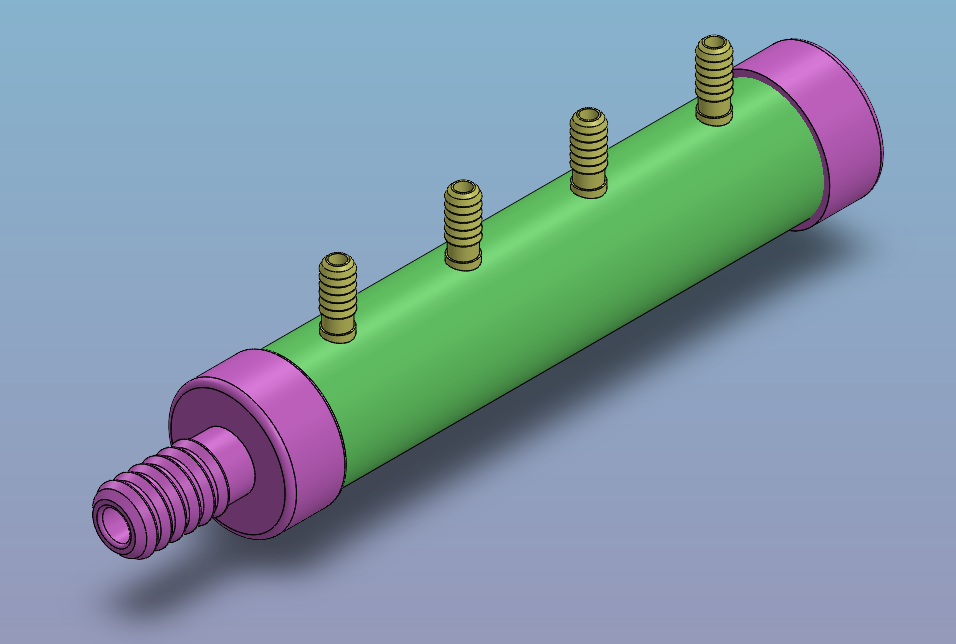
I have made a model of a simple distribution manifold that uses the same pipe that Fredrik uses to build the pistons from, with 3D printed endcaps that allow the flow that we want. the caps can be glued on using 2part epoxy glue that has already been purchased, and the rest should be producable by us.
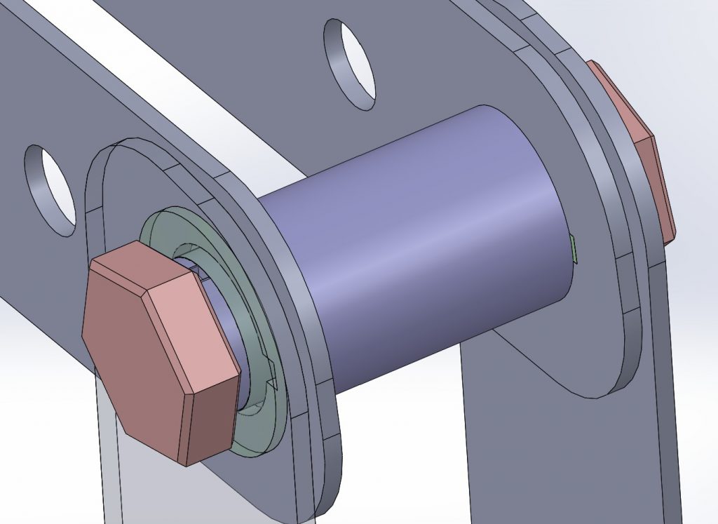
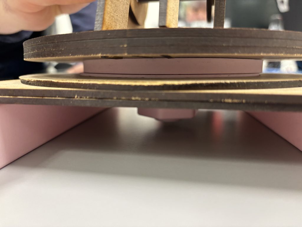
The image below shows the assembly as lasercut and assembled. This was a dry fit, so we hadn’t glues all the plates to each other yet. In this picture the BB pellets are also missing in the bearings.
That’s all for now, see you next week!